Chapter 1: The Vitals of Data

Chapter 1: The Vitals of Data#

Understanding Study Design and Levels of Measurement#

Unit: 1 | Part: I — Describing the World in Numbers

Datasets:

Framingham Heart Study teaching subset (framingham_teaching.csv, n = 500) — Observational

Anorexia Clinical Trial (anorexia via MASS package, n = 72) — Experimental

Learning Objectives

By the end of this chapter, you will be able to:

Differentiate between observational and experimental study designs
Distinguish between categorical and continuous data
Identify the four levels of measurement: nominal, ordinal, interval, and ratio
Classify every variable in our datasets at the correct level
Load the datasets in PSPP and R and inspect their structure

Why This Chapter Comes First#

Before calculating a single mean or p-value, you must answer two fundamental questions: How was this data collected? and What kind of data do I actually have?

This is not housekeeping. It determines every statistical test you can legitimately run. Apply the wrong test to the wrong data type and the software will still produce a number — it will simply be mathematically meaningless.

Observational vs. Experimental Design#

In public health, data generally comes from one of two study designs, both of which we will use throughout this book:

1. Observational Epidemiology (The Framingham Heart Study)

The Method: Researchers observe participants over time without intervening. They measure variables (like blood pressure or smoking habits) and wait to see who develops disease.
The Goal: To identify risk factors and understand how a disease develops naturally.
The Limitation: We can find strong associations, but proving direct cause-and-effect is difficult because we do not control the environment.

2. Experimental Epidemiology (The Anorexia Clinical Trial)

The Method: Researchers actively intervene. Patients are assigned to different groups (e.g., standard care, Cognitive Behavioral Therapy, Family Therapy).
The Goal: To test the effectiveness of a specific treatment or cure.
The Strength: Because researchers control the intervention, this design provides the strongest evidence for cause-and-effect.

Whether you are watching a disease progress or testing a psychological therapy, the next step is looking at the actual measurements. A systolic blood pressure of 0 mmHg means cardiac arrest. An education level of 0 means something entirely different. Getting that distinction right is where all analysis begins.

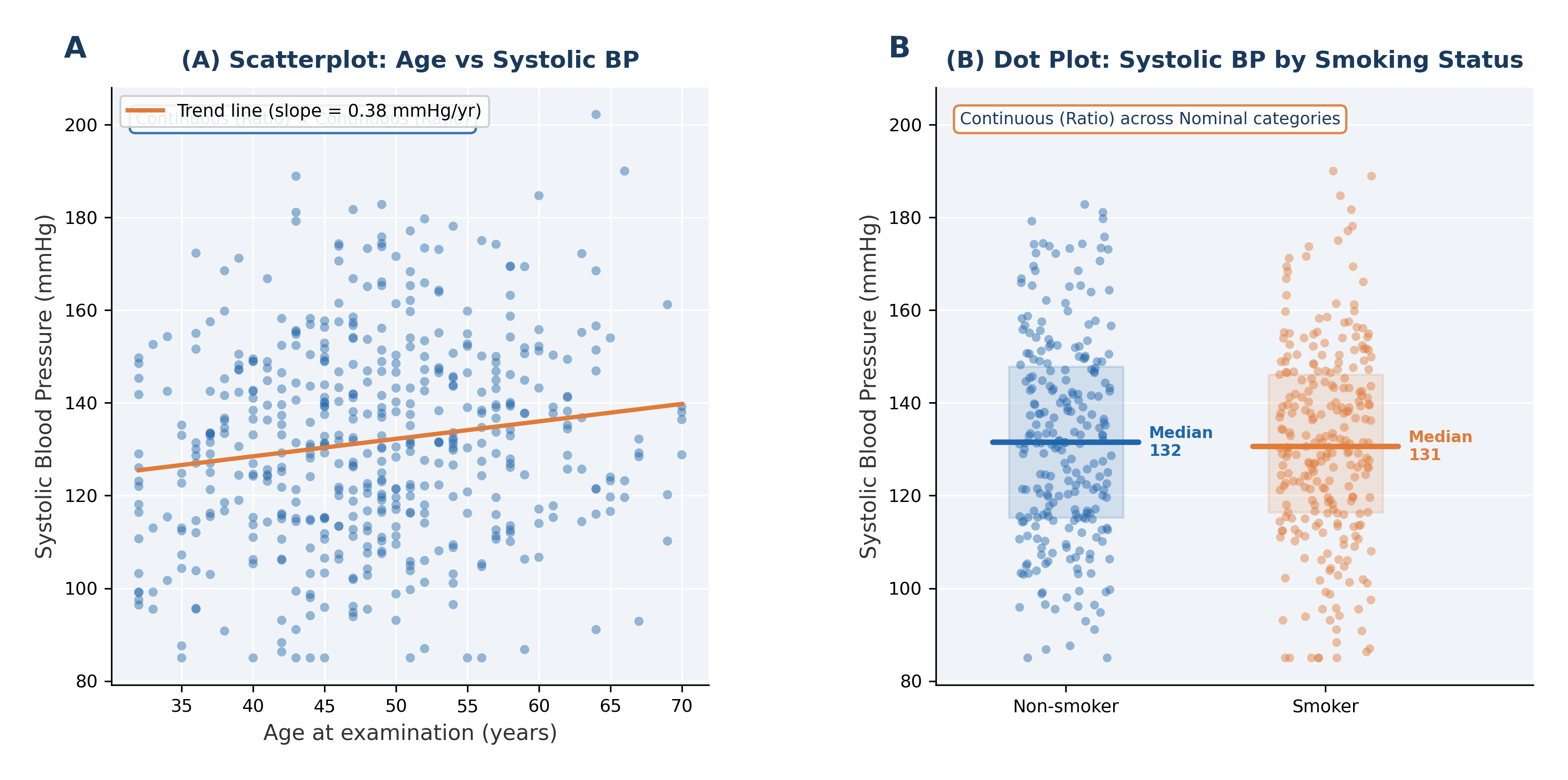
../_images/ch01_framingham_intro.png — Fig. 1 **Figure 1.1 Visualising Relationships and Distributions in the Framingham Study.** These two graphs illustrate foundational concepts in Chapter 1. (A) Scatterplot of Systolic Blood Pressure vs. Age reveals a pattern in two continuous (Ratio) variables, suggesting as Age increases, BP tends to rise. (B) A grouped dot plot contrasts the distribution of Systolic BP (Ratio variable) across two Nominal categories: non-smokers and smokers.#

Section 1: The Two Families of Data#

All health data belongs to one of two families: categorical or continuous.

1.1 Categorical Data#

Categorical data places each observation into a named group. The values do not represent measurable quantities — arithmetic on them is meaningless.

Key diagnostic question: Can I calculate a meaningful average of this variable? If no → categorical.

Examples:

SEX (Framingham) — 1 = Male, 2 = Female. The average of 1 and 2 is 1.5, representing no actual person.
Treat (Anorexia) — CBT, FT, or Cont (Control). Three distinct therapy groups.
CURSMOKE (Framingham) — 0 = non-smoker, 1 = current smoker. Two categories, not quantities.
ANYCHD (Framingham) — did a coronary heart disease event occur during follow-up? 0 = No, 1 = Yes.
DIABETES (Framingham) — 0 = no diabetes, 1 = diabetes present.

⚡ Common mistake: Storing a category as a number does not make it numeric. SEX = 2 does not mean “two units of femaleness.” Always convert categorical variables to factors in R before analysis.

1.2 Nominal Data#

💡 Plain English first: Nominal data is just names for groups — no ranking, no scale, no arithmetic. The only sensible question is “which group appears most?”

Nominal data has categories with no natural order or ranking.

Property	Nominal data
Categories exist	✓ Yes
Natural rank or order	✗ No
Measurable distances	✗ No
True zero	✗ No

Examples: SEX, CURSMOKE, DIABETES, BPMEDS, ANYCHD, DEATH, STROKE (Framingham); Treat (Anorexia).

A common error to avoid: ANYCHD is coded 0 and 1. A student who calculates the mean ANYCHD and reports “0.31” as a statistic is not wrong — this is a proportion (31% had a CHD event). But interpreting 0.31 as an “average CHD level” would be meaningless. The mean of a binary 0/1 variable gives you a proportion, not a numerical average.

1.3 Ordinal Data#

Ordinal data has categories that do have a natural rank order, but the distances between ranks are not equal.

Property	Ordinal data
Categories exist	✓ Yes
Natural rank order	✓ Yes
Equal distances between ranks	✗ No
True zero	✗ No

Framingham example:

EDUC — education level: 1 = 0–11 years, 2 = High school/GED, 3 = Some college, 4 = College graduate or higher.

The rank order is meaningful — Level 4 represents more education than Level 1. But the gap between Level 1 and Level 2 (completing high school) is not the same magnitude as the gap between Level 3 and Level 4 (completing a college degree). We cannot say a Level 4 person has “twice the education” of a Level 2 person.

Other clinical examples:

Cancer staging: Stage I, II, III, IV — ranked, but not equally spaced.
Pain severity: Mild, Moderate, Severe — ranked, gaps unequal.
Glasgow Coma Scale (3–15) — ranked scores, but clinical meaning of each increment differs.

The critical insight: With ordinal data, you know the direction of a difference but not its size.

1.4 Continuous Data#

Continuous data records a genuine numerical measurement where arithmetic operations produce meaningful results.

Key diagnostic question: Does this number represent a real measurement where the gaps between values are equal and meaningful? If yes → continuous.

Examples:

SYSBP (Framingham) — systolic blood pressure in mmHg. 140 mmHg is genuinely higher than 120 mmHg by exactly 20 mmHg.
TOTCHOL (Framingham) — total cholesterol in mg/dL.
Prewt / Postwt (Anorexia) — body weight in pounds.
AGE (Framingham) — age in years at examination.
BMI (Framingham) — body mass index in kg/m².

1.5 Interval Data#

Interval data has equal, meaningful distances between values, but no true zero point. Zero does not mean complete absence of the quantity.

Property	Interval data
Equal distances	✓ Yes
True zero	✗ No
Ratios meaningful	✗ No

Examples:

Temperature in °C: 0 °C is not “no temperature” — it is an arbitrary reference point. 40 °C is not twice as hot as 20 °C.
Calendar year: Year 0 does not mean “no time.” You cannot say 2024 is “twice as recent” as 1012.
Standardised test scores: A score of 0 does not mean zero knowledge.

In the Framingham dataset, the year of birth (derivable from age and study start year) is interval — equal annual gaps, but no true year zero.

1.6 Ratio Data#

Ratio data has equal gaps and a true zero — a zero that genuinely means complete absence.

Property	Ratio data
Equal distances	✓ Yes
True zero	✓ Yes
Ratios meaningful	✓ Yes

⚡ Common mistake: Ask: does zero mean complete absence? Temperature 0°C ≠ no temperature (interval). Blood pressure 0 mmHg = cardiac arrest, no measurable pressure (ratio). Age 0 = newborn (ratio).

Examples:

SYSBP: 0 mmHg = no measurable blood pressure. 160 mmHg is twice 80 mmHg. ✓ Ratio.
AGE: 0 years = newborn. Age 60 is twice as long a life as age 30. ✓ Ratio.
BMI: 0 kg/m² = no body mass. 30 is 1.5× the value of 20. ✓ Ratio.
CIGPDAY: 0 cigarettes = does not smoke at all. ✓ Ratio.
Prewt: 0 lbs = no body weight. ✓ Ratio.

Why this matters clinically: Systolic blood pressure is ratio data. Saying “this patient’s BP is twice the normal value” is a legitimate and clinically actionable ratio statement. The value 0 mmHg is medically unambiguous. Treating BP as interval data would make such ratio statements invalid.

Section 2: The Four Levels — Quick Reference#

Level	Order?	Equal distances?	True zero?	Examples
Nominal	No	No	No	`SEX`, `CURSMOKE`, `ANYCHD`, `Treat`
Ordinal	Yes	No	No	`EDUC` (education level 1–4)
Interval	Yes	Yes	No	Year of birth; temperature
Ratio	Yes	Yes	Yes	`AGE`, `SYSBP`, `BMI`, `TOTCHOL`, `Prewt`

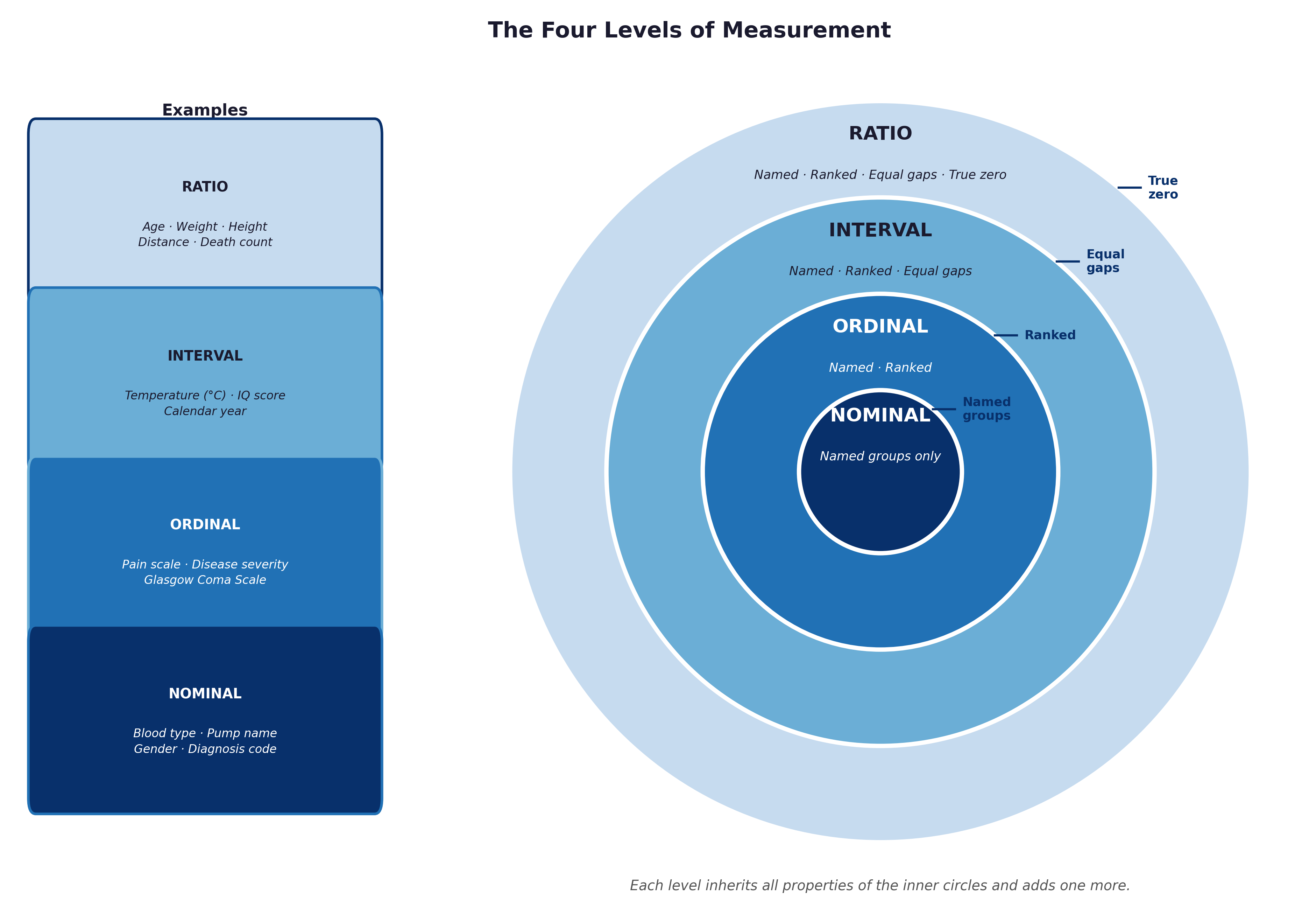
../_images/ch01_levels_of_measurement.png — Fig. 2 **Figure 1.2** The four levels of measurement as nested layers. Each level inherits all properties of those below it and adds exactly one new property.#

The diagnostic shortcut: If you can multiply two values and the result makes clinical sense (“this patient’s BP is twice normal”), the variable is ratio. If only subtraction is meaningful, it is interval. If the numbers are ranks with unequal gaps, it is ordinal. If the values are simply labels, it is nominal.

Section 3: Why Getting This Wrong Causes Real Harm#

Scenario A — Nominal coded as numbers: EDUC is coded 1, 2, 3, 4. A researcher calculates a mean education of 2.1 and reports “the average participant had between high school and some college education.” This is borderline — ordinal data treated as interval. The mean assumes equal gaps between levels, which is almost certainly untrue.

Scenario B — Ordinal treated as interval: Cancer stage (I–IV) is entered as 1–4. A mean stage of 2.3 is reported. The gap between Stage I and II is not clinically equivalent to the gap between Stage III and IV. The mean misleads.

Scenario C — Interval treated as ratio: A researcher says patients examined in 1968 were “twice as recent” as those examined in 984 CE. Nonsense — calendar year has no true zero, so ratios are invalid.

Section 4: Classifying the Datasets#

1. The Anorexia Clinical Trial

Variable	Description	Level	Reasoning
`Treat`	Therapy group	Nominal	Three unordered categories (CBT, FT, Cont)
`Prewt`	Baseline weight (lbs)	Ratio	0 lbs = no mass; ratio valid
`Postwt`	Follow-up weight (lbs)	Ratio	0 lbs = no mass; ratio valid

2. The Framingham Heart Study

Variable	Description	Level	Reasoning
`RANDID`	Participant ID number	Nominal	A label — ID 1050 is not “more” than ID 1025
`SEX`	1=Male, 2=Female	Nominal	Two unordered categories
`EDUC`	Education level 1–4	Ordinal	Ranked but unequal gaps between levels
`AGE`	Age at exam (years)	Ratio	0 = newborn; 60 is twice 30
`CURSMOKE`	Current smoker 0/1	Nominal	Binary category
`CIGPDAY`	Cigarettes per day	Ratio	0 = does not smoke; 20 is twice 10
`TOTCHOL`	Total cholesterol (mg/dL)	Ratio	0 = no cholesterol detectable; ratio valid
`SYSBP`	Systolic BP (mmHg)	Ratio	0 = no measurable pressure; ratio valid
`DIABP`	Diastolic BP (mmHg)	Ratio	Same as SYSBP
`BPMEDS`	On BP medication 0/1	Nominal	Binary category
`DIABETES`	Diabetes present 0/1	Nominal	Binary category
`BMI`	Body mass index (kg/m²)	Ratio	0 = no body mass; ratio valid
`HEARTRTE`	Heart rate (bpm)	Ratio	0 bpm = cardiac arrest; ratio valid
`GLUCOSE`	Blood glucose (mg/dL)	Ratio	0 = no detectable glucose; ratio valid
`PREVCHD`	Prevalent CHD at baseline	Nominal	Binary category
`PREVHYP`	Prevalent hypertension	Nominal	Binary category
`ANYCHD`	Incident CHD during follow-up	Nominal	Binary outcome
`TIMECHD`	Days to CHD event or censoring	Ratio	0 days = event on day of entry
`DEATH`	Death during follow-up	Nominal	Binary outcome
`TIMEDTH`	Days to death or censoring	Ratio	Time is ratio
`STROKE`	Incident stroke	Nominal	Binary outcome
`TIMESTRK`	Days to stroke or censoring	Ratio	Time is ratio

🔬 Lab Manual — Chapter 1#

Objective#

Load the datasets in PSPP and R. Assign the correct variable types and measurement levels. Perform a first inspection of the data structure.

Option A — PSPP (Framingham Data)#

Open PSPP → File → New → Data.
Click the Variable View tab.
Define key variables:

Variable	Type	Measure
`RANDID`	Numeric	Nominal
`SEX`	Numeric	Nominal
`EDUC`	Numeric	Ordinal
`AGE`	Numeric	Scale
`CURSMOKE`	Numeric	Nominal
`CIGPDAY`	Numeric	Scale
`TOTCHOL`	Numeric	Scale
`SYSBP`	Numeric	Scale
`DIABP`	Numeric	Scale
`BMI`	Numeric	Scale
`DIABETES`	Numeric	Nominal
`ANYCHD`	Numeric	Nominal
`DEATH`	Numeric	Nominal

Note: PSPP uses Scale for both interval and ratio variables. Use Nominal for all 0/1 coded variables. Use Ordinal for EDUC.

Import the CSV: File → Import Data → CSV.
Save as framingham_study.sav.

Option B — R / RStudio (Both Datasets)#

# -------------------------------------------------------
# Chapter 1 Lab: Loading the Datasets
# -------------------------------------------------------

# --- PART 1: The Observational Dataset (Framingham) ---
fram_data <- read.csv("data/framingham_teaching.csv")

# First look
head(fram_data)
nrow(fram_data)   # Should be 500
ncol(fram_data)   # Should be 22

# Check the structure — what types has R assigned?
str(fram_data)

# Summary statistics for all variables
summary(fram_data)

# Convert categorical variables to properly labelled factors
fram_data$SEX <- factor(fram_data$SEX,
  levels = c(1, 2), labels = c("Male", "Female"))

fram_data$EDUC <- factor(fram_data$EDUC,
  levels = c(1, 2, 3, 4),
  labels = c("0-11yrs", "HS_GED", "Some_college", "College_grad"),
  ordered = TRUE)   # ordered=TRUE marks it as ordinal

fram_data$CURSMOKE <- factor(fram_data$CURSMOKE,
  levels = c(0, 1), labels = c("Non-smoker", "Smoker"))

fram_data$DIABETES <- factor(fram_data$DIABETES,
  levels = c(0, 1), labels = c("No", "Yes"))

fram_data$ANYCHD <- factor(fram_data$ANYCHD,
  levels = c(0, 1), labels = c("No_event", "CHD_event"))

fram_data$DEATH <- factor(fram_data$DEATH,
  levels = c(0, 1), labels = c("Survived", "Died"))

# Verify
str(fram_data)
summary(fram_data$EDUC)     # Should show ordered factor with 4 levels
summary(fram_data$ANYCHD)   # Should show counts for each outcome

# --- PART 2: The Experimental Dataset (Anorexia) ---
# The anorexia dataset is built directly into the MASS package.
library(MASS)
data(anorexia)

# The 'Treat' variable is already a factor, but let's check the structure
str(anorexia)
summary(anorexia)

What to look for:

After conversion, str() should show SEX, CURSMOKE, DIABETES, ANYCHD, DEATH as Factor.
EDUC should show as Ord.factor — an ordered factor.
AGE, SYSBP, BMI, TOTCHOL should remain int or num.
summary(fram_data$SYSBP) shows min, quartiles, mean, max. What is the median systolic BP in this cohort? Is it above the clinical threshold of 120 mmHg?
In the Anorexia data, Treat should show as a Factor with 3 levels, and weights as numeric.

🧪 Test Your Knowledge#

The variable EDUC is stored as integers 1, 2, 3, 4. A student calculates the mean EDUC and gets 2.1, reporting “the average participant had between high school and some college.” (a) What level of measurement is EDUC? (b) Is calculating the mean valid here? (c) What would be a more appropriate summary statistic?

Key Terms#

Term	Definition
Observational design	Studying a population without active intervention to find risk factors.
Experimental design	Actively intervening to test the efficacy of a treatment (e.g., a clinical trial).
Categorical data	Data placing observations into named groups; arithmetic is not meaningful.
Continuous data	Data measured on a numerical scale; arithmetic operations produce valid results.
Nominal	Categories with no natural order. Examples: `SEX`, `CURSMOKE`, `ANYCHD`, `Treat`.
Ordinal	Ranked categories with unequal gaps. Example: `EDUC` (education level 1–4).
Interval	Numerical scale with equal gaps but no true zero. Example: calendar year.
Ratio	Numerical scale with equal gaps and a true zero. Examples: `AGE`, `SYSBP`, `BMI`, `Prewt`.
Level of measurement	The classification of a variable that determines which mathematical operations are legitimate.
True zero	A zero value representing complete absence of the measured quantity.

Review Questions#

Explain the primary difference between observational epidemiology (like Framingham) and experimental epidemiology (like the Anorexia trial).
Classify each Framingham variable at the correct level of measurement and justify your answer: HEARTRTE, GLUCOSE, BPMEDS, CIGPDAY, EDUC.
ANYCHD is stored as 0 and 1. A student calculates the mean ANYCHD across all 500 participants and gets 0.31. (a) What does this number mean? (b) Is calculating the mean of a 0/1 variable meaningful? (c) What is the correct level of measurement for ANYCHD?
A hospital records each patient’s diastolic blood pressure in mmHg. Classify this variable at the correct level and justify every step.
Explain why EDUC (education level 1–4) is ordinal rather than interval. Give a specific example of an interval statement that would be invalid for this variable.
In R, after loading the dataset, run str(fram_data). Which variables does R initially classify as int that should actually be treated as nominal or ordinal factors? Write the code to correct each one.
A researcher averages the EDUC scores across all participants and reports “mean education = 2.1.” Another researcher reports “the modal education level is ‘0–11 years’ (Level 1), seen in 193/500 participants.” Which summary is more appropriate and why?

Key Takeaways

Study Design: Observational watches for risks; Experimental tests interventions.
Two data families: Categorical (named groups) vs. Continuous (measurable quantities).
Four levels: Nominal → Ordinal → Interval → Ratio. Each adds one property.
Framingham dataset: SEX, CURSMOKE, DIABETES, ANYCHD, DEATH = nominal; EDUC = ordinal; AGE, SYSBP, BMI, TOTCHOL = ratio.
Common error: Numeric storage ≠ numeric meaning. Always convert categorical variables to factors in R.
Ratio vs interval: Ask — does zero mean complete absence? BP 0 = cardiac arrest (ratio). Year 0 = arbitrary reference (interval).

Next: Chapter 2 — The Middle and the Mess uses the ratio variables to calculate the descriptive statistics that characterise our datasets.

Part I — Describing the World in Numbers

Chapter 1: The Vitals of Data

Contents

Chapter 1: The Vitals of Data#

Understanding Study Design and Levels of Measurement#

Why This Chapter Comes First#

Observational vs. Experimental Design#

Section 1: The Two Families of Data#

1.1 Categorical Data#

1.2 Nominal Data#

1.3 Ordinal Data#

1.4 Continuous Data#

1.5 Interval Data#

1.6 Ratio Data#

Section 2: The Four Levels — Quick Reference#

Section 3: Why Getting This Wrong Causes Real Harm#

Section 4: Classifying the Datasets#

🔬 Lab Manual — Chapter 1#

Objective#

Option A — PSPP (Framingham Data)#

Option B — R / RStudio (Both Datasets)#

🧪 Test Your Knowledge#

Key Terms#

Review Questions#