Chapter 2: The Middle and the Mess#
Measures of Central Tendency and Variability#
Dataset: Framingham Heart Study teaching subset —
framingham_teaching.csv, n = 500 participants, baseline examination.
Learning Objectives
By the end of this chapter, you will be able to:
Calculate and interpret the mean, median, and mode.
Calculate the range, interquartile range (IQR), variance (with Bessel’s correction), and standard deviation.
Choose the correct measure of central tendency based on distribution shape.
Produce and interpret descriptive statistics in PSPP and R.
Before You Begin: Why Summaries Matter#
500 rows of blood pressure readings, cholesterol values, and smoking histories tell the human brain almost nothing actionable. A physician cannot treat a spreadsheet. A public health officer cannot design a hypertension intervention from 500 individual numbers.
To make decisions, we compress data into two questions:
Where is the centre? — Central tendency (mean, median, mode)
How spread out is it? — Variability (range, IQR, variance, standard deviation)
For the Framingham cohort, these questions have immediate clinical meaning. What is the typical systolic blood pressure of a middle-aged American in the 1950s? How widely does cholesterol vary across the population? These statistical summaries form the foundation of every cardiovascular risk guideline used today.
Section 1: Finding the Centre — Central Tendency#
1.1 The Mean#
💡 Plain English first: Add all the values together and divide by how many there are. The result is heavily pulled toward any extreme values in the data.
The mean (\(\bar{x}\), pronounced “x-bar”) is the arithmetic average.
Worked example — systolic blood pressure: Seven participants have systolic BPs (mmHg): 118, 135, 122, 148, 110, 165, 128.
When to use the mean: Continuous, ratio/interval-level data that is approximately symmetrically distributed (bell-shaped).
⚠️ Sensitivity to outliers: A single participant with a hypertensive crisis (e.g., 220 mmHg) will drag the mean upward. In a population where 95% of participants have a systolic BP between 100 and 170 mmHg, that one extreme value makes the “average” appear higher than what most people actually experience.
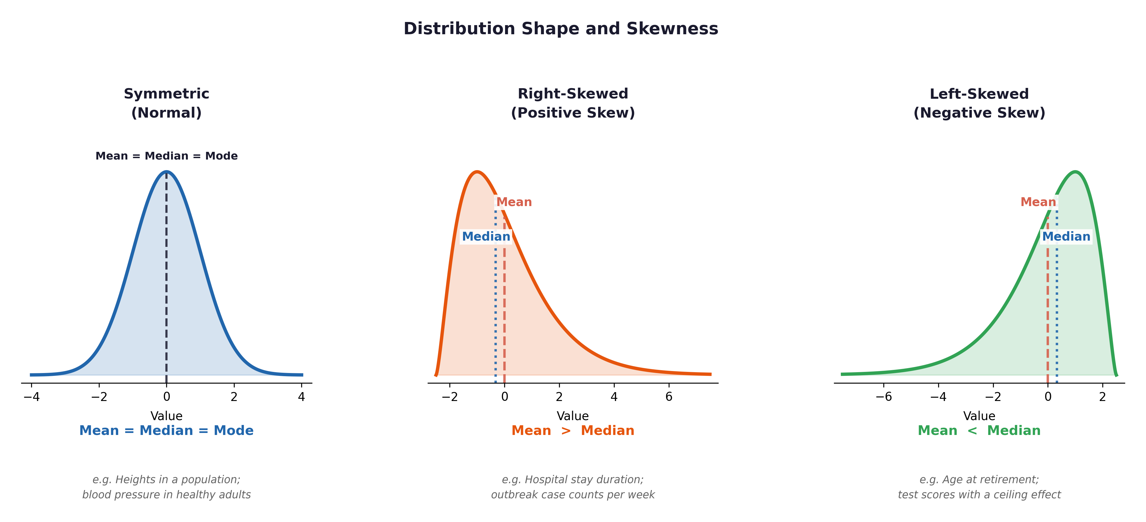
Fig. 3 Figure 2.1 Symmetric, right-skewed, and left-skewed distributions. Systolic blood pressure tends to be slightly right-skewed — most participants cluster in a normal range, but hypertensive outliers create a long right tail. When the mean substantially exceeds the median, report the median.#
1.2 The Median#
The median is the exact middle value when all observations are ranked in ascending order.
If \(n\) is odd: The value at position \(\frac{n+1}{2}\)
If \(n\) is even: The average of the two middle values
Worked example: Seven BPs ranked: 110, 118, 122, 128, 135, 148, 165. \(n = 7\) (odd) \(\rightarrow\) median is at position 4 \(\rightarrow\) 128 mmHg.
Notice that the outlier of 165 has absolutely no effect on the median. The median would remain 128 mmHg whether that last participant had a BP of 165 or 265.
When to use the median in cardiovascular epidemiology:
Cholesterol (tends to be right-skewed in population samples)
Cigarettes per day (heavily right-skewed — many non-smokers, a few heavy smokers)
Glucose levels (right-skewed — most are normal, a few are diabetic outliers)
Time-to-event variables (always use median survival time, never mean)
1.3 The Mode#
The mode is the most frequently occurring value. It is the only measure of central tendency that is valid for nominal (categorical) data.
Framingham examples:
Modal
SEX= Female (57% of the sample)Modal
EDUC= Level 1 (0–11 years of schooling) — 193 out of 500 participantsModal
CURSMOKE= Smoker (51% at baseline — reflecting 1950s smoking prevalence)
For a nominal variable like ANYCHD (0 = no event, 1 = event), calculating a mean or median is mathematical nonsense. The mode simply tells us: the most common outcome in the Framingham cohort was no CHD event (69% of the sample).
1.4 Choosing the Right Measure#
Situation |
Best Measure |
Reason |
|---|---|---|
Continuous, symmetric data |
Mean |
Uses every value; mathematically powerful for later tests. |
Continuous, skewed data |
Median |
Resistant to distortion by extreme outliers. |
Nominal categorical data |
Mode |
Categories cannot be mathematically added or ranked. |
Ordinal data |
Median or Mode |
Ordinal data has rank, but the distances between ranks are not equal. |
Section 2: Measuring the Mess — Variability#
Two different Framingham cohorts with the exact same mean systolic BP could have vastly different clinical implications—one might be tightly clustered around 130 mmHg, while the other contains many dangerous hypertensive extremes. Measures of variability capture that spread.
2.1 The Range#
Framingham example: If the highest SYSBP in the dataset is 228 mmHg and the lowest is 83.5 mmHg, the range is 144.5 mmHg.
Limitation: The range uses only the two most extreme data points. If 498 participants have a SYSBP between 100–160 mmHg, but two extreme outliers exist, the range heavily exaggerates the spread of the data.
2.2 Quartiles and the Interquartile Range (IQR)#
Because the range is so easily distorted, we often divide the ranked data into four equal parts (quartiles).
Q1 (25th percentile): 25% of the data falls below this value.
Q2 (50th percentile): The Median.
Q3 (75th percentile): 75% of the data falls below this value.
The Interquartile Range (IQR) is the distance between Q1 and Q3 (\(IQR = Q3 - Q1\)). It represents the “middle 50%” of your data, making it a highly robust measure of spread that completely ignores extreme outliers.
Epidemiologists use the IQR to mathematically define outliers. Any value that sits more than 1.5 × IQR above Q3 or below Q1 is flagged as an outlier. This is exactly how the “whiskers” and “dots” on a box plot are drawn.
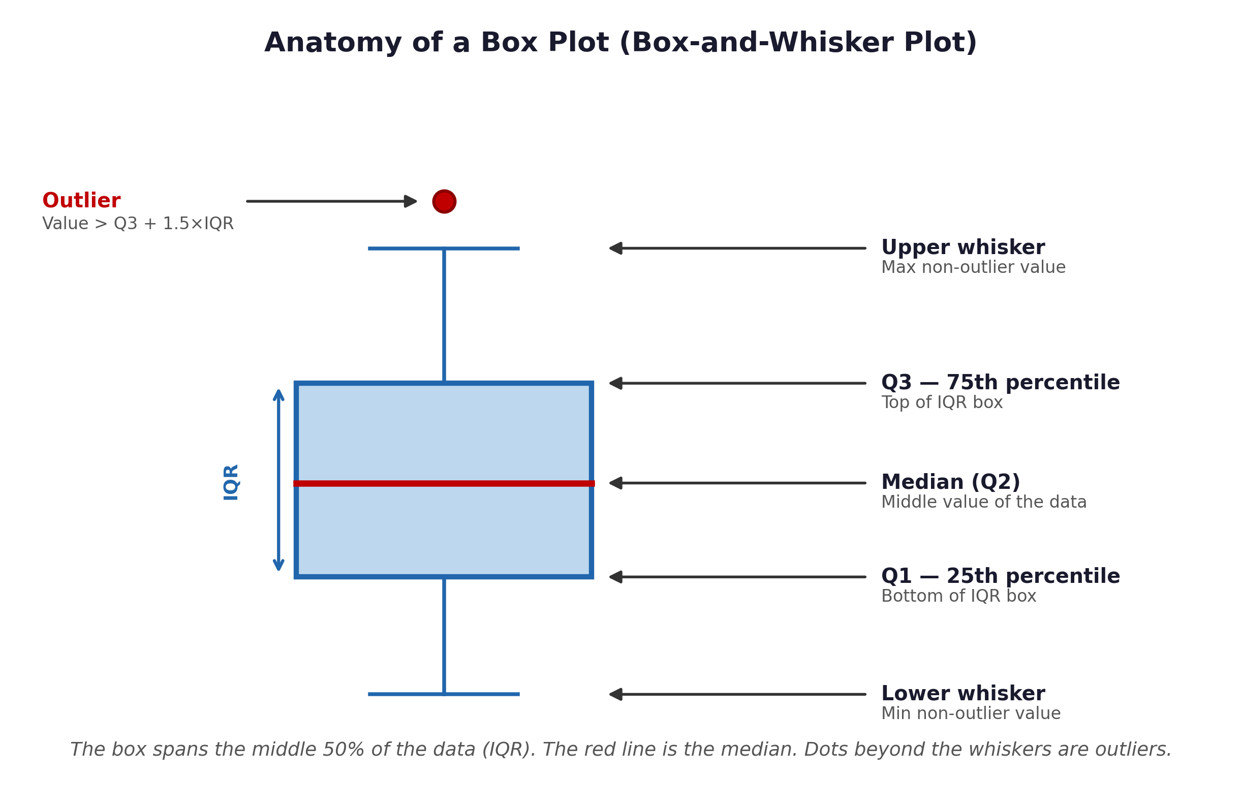
Fig. 4 Figure 2.2 Anatomy of a box plot. The box spans the middle 50% of the data (IQR = Q3 − Q1). The red line is the median. Whiskers extend to the maximum and minimum values that are not outliers. Dots beyond the whiskers represent true mathematical outliers (> 1.5 × IQR from the box edges). In the Framingham dataset, a box plot of SYSBP would show the median around 128 mmHg with a right-skewed distribution.#
2.3 Variance#
💡 Plain English first: Variance asks — on average, how far does each individual blood pressure reading sit from the overall mean? It measures spread in “squared” units.
Why (n − 1)? Our 500 participants are just a sample drawn from the larger population of all middle-aged Americans. Mathematically, dividing by \(n\) slightly underestimates the true variability of that wider population. Dividing by \((n - 1)\) corrects this underestimation. This is known as Bessel’s correction.
⚡ Common mistake: Students often ask why we square the deviations rather than just taking the absolute value. While both work conceptually, squaring the numbers gives variance much cleaner algebraic properties, making it the standard engine behind all advanced parametric statistics (like ANOVA and Regression).
2.4 Standard Deviation#
The standard deviation (\(s\)) simply takes the square root of the variance, returning the measurement of spread back to the original, readable units (e.g., mmHg instead of mmHg²).
A small SD means BPs cluster tightly around the mean; the cohort is homogeneous.
A large SD means BPs scatter widely; the cohort spans a broad clinical range.
2.5 Worked Example — Cholesterol Variance#
Seven participants’ total cholesterol readings (mg/dL): 195, 220, 245, 210, 280, 230, 215. The Mean (\(\bar{x}\)) = 227.9 mg/dL.
\(x_i\) |
Deviation (\(x_i - \bar{x}\)) |
Squared Deviation \((x_i - \bar{x})^2\) |
|---|---|---|
195 |
−32.9 |
1082.4 |
220 |
−7.9 |
62.4 |
245 |
+17.1 |
292.4 |
210 |
−17.9 |
320.4 |
280 |
+52.1 |
2714.4 |
230 |
+2.1 |
4.4 |
215 |
−12.9 |
166.4 |
Sum |
0.0 |
4642.8 |
Note: The sum of the raw deviations always equals exactly zero — the positive and negative deviations cancel each other out. This is why we must square them!
Interpretation: The typical participant’s cholesterol is about 227.9 mg/dL, and individual values typically deviate from that mean by about 27.8 mg/dL. At the population level, a clinical guideline threshold of 240 mg/dL sits less than one standard deviation above the mean — suggesting that a substantial fraction of the Framingham cohort was already at or near elevated cardiovascular risk.
Section 3: Descriptive Statistics and Clinical Interpretation#
Descriptive statistics are almost always reported together. A mean alone is incomplete; the mean combined with its standard deviation tells the full clinical story.
Variable |
Mean ± SD |
Median |
Clinical Interpretation |
|---|---|---|---|
AGE |
48.4 ± 8.7 years |
48 years |
A middle-aged cohort; ages range from 32–70. |
SYSBP |
131.6 ± 21.9 mmHg |
~128 mmHg |
Mean is above normal (120); distribution is right-skewed. |
TOTCHOL |
235 ± 42 mg/dL |
~232 mg/dL |
Mean is approaching the “borderline high” threshold of 240. |
BMI |
26.0 ± 4.4 kg/m² |
~25.6 kg/m² |
Mean sits in the overweight range (25.0–29.9). |
CIGPDAY |
(Right-skewed) |
0 (Non-smoker) |
51% smoke; among the smokers, there is a very wide range. |
🔬 Lab Manual — Chapter 2#
Objective#
Calculate descriptive statistics for SYSBP, TOTCHOL, AGE, and BMI. Identify which variables are skewed and why.
Option A — PSPP#
To get a complete table of mean, median, standard deviation, and range in one step:
Open
framingham_teaching.csv.Go to Analyze → Descriptive Statistics → Frequencies.
Move
SYSBP,TOTCHOL,AGE, andBMIinto the Variables box.Click Statistics…
Check the boxes for Mean, Median, Mode, Std. deviation, Minimum, and Maximum.
Click Continue, then OK.
Option B — R / RStudio#
# -------------------------------------------------------
# Chapter 2 Lab: Descriptive Statistics
# Dataset: framingham_teaching.csv
# -------------------------------------------------------

fram_data <- read.csv("data/framingham_teaching.csv")

# ── Descriptives for key continuous variables ─────────
vars <- c("SYSBP", "TOTCHOL", "AGE", "BMI", "CIGPDAY", "GLUCOSE")

for (v in vars) {
  cat("\n──", v, "──\n")
  cat("  Mean:  ", round(mean(fram_data[[v]],   na.rm=TRUE), 2), "\n")
  cat("  Median:", median(fram_data[[v]],        na.rm=TRUE), "\n")
  cat("  SD:    ", round(sd(fram_data[[v]],      na.rm=TRUE), 2), "\n")
  cat("  Range: ", range(fram_data[[v]],         na.rm=TRUE), "\n")
}

# ── Summary for all variables (Includes IQR Quartiles) ──
summary(fram_data)

# ── Mode for categorical variables ───────────────────
fram_data$SEX      <- factor(fram_data$SEX, levels=c(1,2), labels=c("Male","Female"))
fram_data$CURSMOKE <- factor(fram_data$CURSMOKE, levels=c(0,1), labels=c("Non-smoker","Smoker"))
fram_data$EDUC     <- factor(fram_data$EDUC, levels=1:4,
                             labels=c("0-11yrs","HS_GED","Some_college","College_grad"),
                             ordered=TRUE)

table(fram_data$SEX)
table(fram_data$CURSMOKE)
table(fram_data$EDUC)

# ── Descriptives separated by smoking group ───────────
tapply(fram_data$SYSBP, fram_data$CURSMOKE, mean,   na.rm=TRUE)
tapply(fram_data$SYSBP, fram_data$CURSMOKE, median, na.rm=TRUE)
tapply(fram_data$SYSBP, fram_data$CURSMOKE, sd,     na.rm=TRUE)

# ── Variance ──────────────────────────────────────────
var(fram_data$TOTCHOL, na.rm=TRUE)
What to examine:
For
SYSBPandTOTCHOL: is the mean close to the median, or does the mean exceed the median (indicating a right skew)?Notice the output from the
summary()function. It explicitly gives you the1st Qu.(Q1) and3rd Qu.(Q3). These are the exact values used to draw the box plot from Figure 2.2!The Standard Deviation (SD) of
SYSBP(\(\approx 22\) mmHg) means that approximately 68% of the participants fall within \(\pm 22\) mmHg of the mean — from about 110 to 154 mmHg.
🧪 Test Your Knowledge#
Compute the mean, median, and SD of TOTCHOL separately for smokers and non-smokers.
(a) Write the R code using tapply().
(b) Is the difference in mean cholesterol clinically meaningful?
(c) Does smoking appear to be associated with higher cholesterol in this sample?
Show Solution
# (a) R code
fram_data$CURSMOKE <- factor(fram_data$CURSMOKE, levels=c(0,1),
  labels=c("Non-smoker","Smoker"))

tapply(fram_data$TOTCHOL, fram_data$CURSMOKE, mean,   na.rm=TRUE)
tapply(fram_data$TOTCHOL, fram_data$CURSMOKE, median, na.rm=TRUE)
tapply(fram_data$TOTCHOL, fram_data$CURSMOKE, sd,     na.rm=TRUE)

# (b) A difference of ~5-10 mg/dL between smokers and non-smokers
#     is modest but directionally consistent with the Framingham literature.
#     Whether it is clinically meaningful depends on the absolute values —
#     if both groups average above 230 mg/dL, the difference matters less
#     than the fact that BOTH groups are approaching the "borderline high"
#     cardiovascular risk threshold.

# (c) We can note a visible association from these descriptive statistics,
#     but we cannot yet determine if it is STATISTICALLY SIGNIFICANT.
#     That requires a formal hypothesis test, which we will cover in Chapter 6.
Key Terms#
Term |
Definition |
|---|---|
Central tendency |
A single value summarising the “centre” of a distribution: mean, median, or mode. |
Mean (\(\bar{x}\)) |
Arithmetic average. Sensitive to outliers; best for symmetric distributions. |
Median |
The exact middle value when ranked. Resistant to outliers; preferred for skewed health data. |
Mode |
The most frequent value. The only valid central tendency measure for nominal data. |
Variability |
The degree to which values spread out around the centre. |
Range |
Maximum − Minimum. Simple to calculate but easily distorted by extreme values. |
Interquartile Range (IQR) |
Q3 − Q1. The spread of the middle 50% of the data. Highly resistant to outliers. |
Variance (\(s^2\)) |
Average squared deviation from the mean. |
Standard deviation (\(s\)) |
\(\sqrt{\text{variance}}\). Measures spread in the original units; highly interpretable. |
Bessel’s correction |
Dividing by \((n-1)\) rather than \(n\) to produce an unbiased estimate of population variance. |
Review Questions#
The Framingham dataset shows a mean SYSBP of 131.6 mmHg and a median of approximately 128 mmHg. What does this tell you about the shape of the distribution? Would you report the mean or the median as the “typical” systolic BP? Justify your answer.
Calculate the mean and standard deviation for these cholesterol values (mg/dL): 180, 210, 225, 240, 195, 310, 220. Show your working. What does the large deviation of the 310 value tell you about the limitations of the mean?
CIGPDAY(cigarettes per day) has a median of 0 and a mean well above 0. Explain why this happens, and state which measure better represents the “typical” smoking level in this specific cohort.Why is neither the mean nor the median appropriate for summarising
ANYCHD? What measure should be used, and what does it reveal?The SD of
TOTCHOLin the Framingham cohort is approximately 42 mg/dL. Using the Empirical Rule (which you will learn more about in Chapter 4), what range of cholesterol values would contain approximately 95% of the participants if cholesterol were perfectly normally distributed?In R, run
tapply(fram_data$BMI, fram_data$SEX, summary). Compare the mean and median BMI by sex. In which group is the BMI more heavily skewed, and how can you mathematically tell?
Key Takeaways
Mean = \(\sum x_i / n\) — sensitive to outliers; best for symmetric distributions (e.g., SYSBP, AGE).
Median = middle value — resistant to outliers; best for skewed data (e.g., CIGPDAY, time-to-event).
Standard Deviation (SD) = \(\sqrt{s^2}\) — measured in the same units as the variable; the most interpretable measure of spread.
Bessel’s correction uses \((n-1)\) to give an unbiased estimate of the true population variance.
The Skewness Rule: If the Mean > Median, you likely have a right (positive) skew.
In R:
mean(),median(),sd(),var(),summary(). In PSPP: Analyze → Descriptive Statistics → Frequencies.
Next: Chapter 3 — The Margin of Error asks how confident we can be that our specific sample statistics actually reflect the broader population of middle-aged Americans.
Part I — Describing the World in Numbers