Chapter 3: The Margin of Error

Chapter 3: The Margin of Error#

Uncertainty, Sampling, and Confidence Intervals#

Dataset: Framingham Heart Study teaching subset — framingham_teaching.csv, n = 500 participants, baseline examination.

Learning Objectives

By the end of this chapter, you will be able to:

Distinguish between a population parameter and a sample statistic.
Calculate the standard error of the mean.
Construct and correctly interpret a 95% confidence interval.
Distinguish random error from systematic bias.

Before You Begin: From Description to Inference#

Chapter 2 described our 500 Framingham participants. But the scientific goal is broader: to use this specific sample to draw conclusions about the wider population — all middle-aged Americans of that era, and by extension, populations at cardiovascular risk today.

This is the shift from descriptive to inferential statistics. It requires accepting one fundamental fact: every sample statistic carries uncertainty. This chapter gives you the mathematical tools to quantify that uncertainty: the standard error and the confidence interval.

Section 1: Populations and Samples#

1.1 Key Definitions#

Population parameter — the true, exact value for the entire population (e.g., the true mean systolic BP of all middle-aged Americans in the 1950s). Denoted by Greek letters like $\mu$ (mean) and $\sigma$ (standard deviation).
Sample statistic — the value calculated from our specific 500 participants. Denoted by Roman letters like $\bar{x}$ (mean) and $s$ (standard deviation).
Sampling error — the inevitable, random difference between a sample statistic and the true population parameter it is trying to estimate. This is not a mistake — it is a mathematical certainty of taking a sample.

Our 500 participants are a sample. Their mean SYSBP ($\bar{x}$) is our best estimate of the population mean ($\mu$), but we know $\bar{x} \neq \mu$ exactly. How far off might our estimate be? The standard error answers this.

1.2 Accuracy vs Precision#

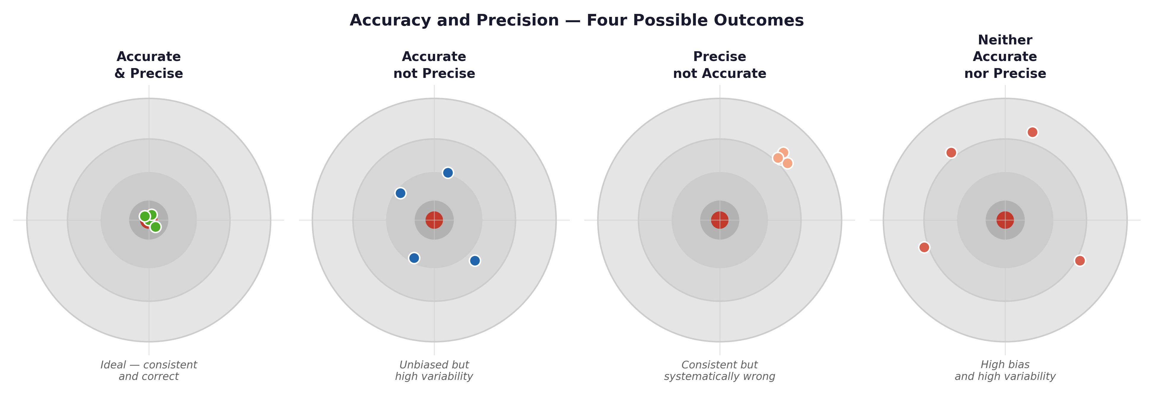
../_images/ch03_accuracy_precision.png — Fig. 5 **Figure 3.1** Accuracy vs precision illustrated with target diagrams. High precision with low accuracy (systematic bias) is more dangerous than low precision alone — it produces confident, reproducible, and consistently wrong results. In epidemiology, a miscalibrated blood pressure cuff produces this pattern.#

Framingham example: If the blood pressure cuffs used in the 1950s Framingham exams were systematically over-reading by 5 mmHg (a calibration error), every measurement would be highly precise (tightly clustered) but completely inaccurate (missing the true bullseye). A larger sample size would not fix this — it would just give you a more precisely wrong answer.

Section 2: The Standard Error#

2.1 Standard Deviation vs Standard Error#

💡 Plain English first: If you drew 100 different random samples of 500 Framingham participants, each sample would give you a slightly different mean SYSBP. The Standard Error (SE) measures how much those sample means typically vary from one another. It is literally the standard deviation of the sample means.

Statistic	What it measures	Formula
Standard Deviation (s)	The spread of individual observations within a single sample.	$$s = \sqrt{\frac{\sum(x_i-\bar{x})^2}{n-1}}$$
Standard Error (SE)	The precision of the sample mean as an estimate.	$$SE = \frac{s}{\sqrt{n}}$$

Worked example — SYSBP:

Mean ($\bar{x}$) = 131.6 mmHg
Standard Deviation (s) = 21.9 mmHg
Sample Size (n) = 500

\[SE = \frac{21.9}{\sqrt{500}} = \frac{21.9}{22.36} \approx 0.98 \text{ mmHg}\]

Our sample mean of 131.6 mmHg estimates the true population mean, and we expect that estimate to be off by about 1 mmHg on average due to random sampling error.

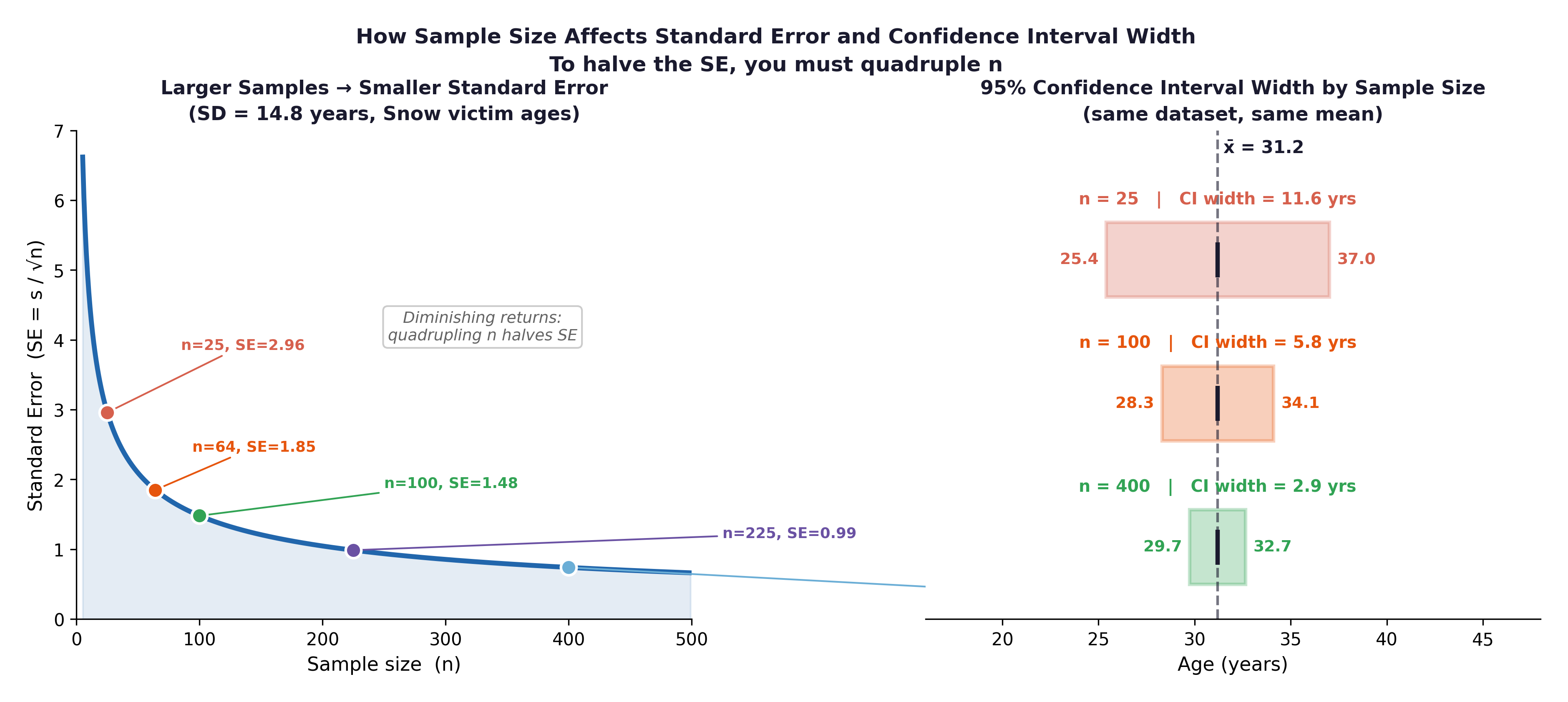
../_images/ch03_sample_size_se.png — Fig. 6 **Figure 3.2** The relationship between sample size and standard error. The Framingham study’s large sample (here n = 500) yields a very small SE; the mean blood pressure estimate is highly precise. Halving the sample to 250 would increase the SE by a factor of $\sqrt{2} \approx 1.41$, not by double.#

Key relationship: SE = s / √n. Because of the square root, to halve your Standard Error, you must quadruple your sample size. This mathematical reality has major implications for clinical trial design — buying precision is very expensive.

Section 3: The 95% Confidence Interval#

3.1 Construction#

To build a 95% Confidence Interval (CI), we take our sample mean and add/subtract a margin of error. For large samples (n ≥ 30), we use the multiplier 1.96 (derived from the Normal distribution).

\[95\% \text{ CI} = \bar{x} \pm 1.96 \times SE\]

Worked example — mean SYSBP: $$95\% \text{ CI} = 131.6 \pm (1.96 \times 0.98)$$95\% \text{ CI} = 131.6 \pm 1.92$$= [129.7 \text{ mmHg}, 133.5 \text{ mmHg}]$$

3.2 Correct Interpretation#

We are 95% confident that the true mean systolic blood pressure in the population from which this sample was drawn is between 129.7 and 133.5 mmHg.

⚡ Common mistake — the two most frequent CI misinterpretations:

❌ “There is a 95% probability that the true mean lies in this interval.” ✅ The 95% refers to the procedure. If we repeated this study 100 times, 95 of the intervals we created would successfully capture the true population mean. This specific interval (129.7 to 133.5) either contains the true mean (100% probability) or it doesn’t (0% probability).

❌ “95% of individual participants have a SYSBP between 129.7 and 133.5 mmHg.” ✅ The CI is about the precision of the mean, not about the spread of individuals. The range of individual blood pressures in our dataset is vastly wider (83.5 to 228.0 mmHg).

3.3 What Affects CI Width?#

Factor	Effect on CI	Clinical Implication
Larger sample size (n)	Narrower	The Framingham study’s massive cohort produced incredibly narrow, precise CIs.
Smaller SD (s)	Narrower	A more biologically homogeneous population yields a more precise mean estimate.
99% vs 95% confidence	Wider	If you want to be more certain you caught the true mean, you must cast a wider net.

3.4 Bias: What a CI Cannot Fix#

A Confidence Interval only quantifies random error (unavoidable sampling variation). It cannot fix systematic bias (a consistent, directional error in how data was collected).

Error Type	Cause	Fixed by a larger sample?	Example
Random error	Sampling variation	✓ Yes (SE shrinks)	Different nurses get slightly different BP readings by chance.
Selection bias	Unrepresentative sample	✗ No	The original Framingham cohort enrolled only White participants.
Information bias	Systematic mismeasurement	✗ No	A miscalibrated blood pressure cuff over-reads by 5 mmHg for everyone.

Epidemiological example: The original Framingham cohort was almost entirely White, drawn from one specific Massachusetts town. The mean SYSBP we calculate may be an incredibly precise estimate of this specific population while simultaneously being a heavily biased estimate of the broader American population. No amount of additional Framingham participants can fix that selection bias.

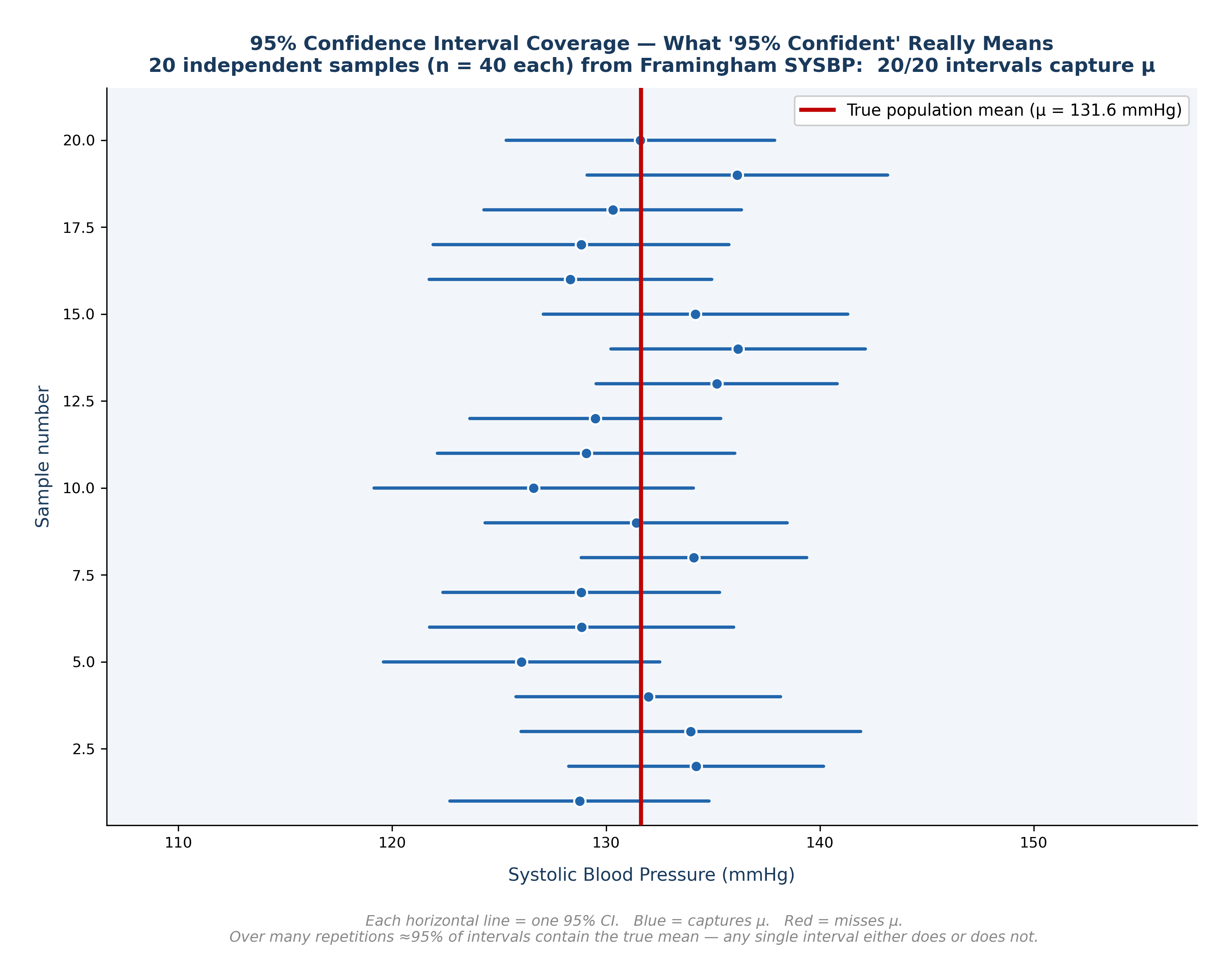
../_images/ch03_ci_coverage.png — Fig. 7 **Figure 3.3 What ‘95% Confident’ Really Means — CI Coverage Diagram.** Twenty independent samples of n = 40 drawn from the Framingham SYSBP data. Each horizontal line is one 95% CI; the dot marks the sample mean. Blue intervals capture the true mean (red line); red intervals miss it. Over many repetitions, approximately 95% of such intervals will contain μ, but any single interval either does or does not.#

🔬 Lab Manual — Chapter 3#

Objective#

Calculate the Standard Error and 95% Confidence Interval for mean SYSBP and TOTCHOL. Compare the CI widths and interpret the results.

Option A — PSPP#

Open framingham_teaching.csv.
Analyze → Compare Means → One-Sample T Test.
Move SYSBP and TOTCHOL to the Test Variables box. Set Test Value = 0.
Click OK. The 95% Confidence Interval will appear in the final output table.

Option B — R / RStudio#

# -------------------------------------------------------
# Chapter 3 Lab: Standard Error and Confidence Intervals
# -------------------------------------------------------

fram_data <- read.csv("data/framingham_teaching.csv")

# ── Manual SE and 95% CI for SYSBP ───────────────────
n     <- length(na.omit(fram_data$SYSBP))
x_bar <- mean(fram_data$SYSBP, na.rm = TRUE)
s     <- sd(fram_data$SYSBP,   na.rm = TRUE)
SE    <- s / sqrt(n)

CI_lower <- x_bar - 1.96 * SE
CI_upper <- x_bar + 1.96 * SE

cat("SYSBP: mean =", round(x_bar,2), "| SD =", round(s,2),
    "| SE =", round(SE,3), "\n")
cat("Manual 95% CI: [", round(CI_lower,2), ",", round(CI_upper,2), "] mmHg\n")

# ── Using t.test() — the standard R method ────────────
# Note: t.test() uses the exact T-distribution multiplier (e.g., 1.964) 
# instead of the rounded 1.96 Normal multiplier, so its CI will be 
# a tiny fraction wider than our manual calculation above. This is normal!

t.test(fram_data$SYSBP)
t.test(fram_data$TOTCHOL)

# ── Compare CI widths ─────────────────────────────────
# Which variable has more uncertainty in its mean estimate?
ci_sysbp <- t.test(fram_data$SYSBP)$conf.int
ci_chol  <- t.test(fram_data$TOTCHOL)$conf.int

cat("SYSBP CI width:  ", round(diff(ci_sysbp), 3), "mmHg\n")
cat("TOTCHOL CI width:", round(diff(ci_chol),  3), "mg/dL\n")

# ── CI for SYSBP separated by smoking group ───────────
by(fram_data$SYSBP,
   factor(fram_data$CURSMOKE, labels=c("Non-smoker","Smoker")),
   function(x) t.test(x)$conf.int)

🧪 Test Your Knowledge#

A clinician reads your report and says: “Your 95% CI for mean SYSBP is [129.7, 133.5] mmHg. That means 95% of your participants have blood pressure in that exact range.” (a) Identify the statistical error. (b) Write the correct interpretation. (c) What is the actual range of individual SYSBP values in this dataset?

Key Terms#

Term	Definition
Population parameter	The true, exact value for the entire population. Denoted $\mu$, $\sigma$.
Sample statistic	The value calculated from a specific sample. Denoted $\bar{x}$, s.
Sampling error	The inevitable random difference between a sample statistic and the population parameter.
Standard error (SE)	SE = s / √n. Measures how precisely the sample mean estimates the population mean.
95% Confidence interval	$\bar{x} \pm 1.96 \times SE$. The plausible range for the true population mean.
Random error	Unavoidable sampling variation. Can be reduced by increasing n.
Systematic bias	Consistent directional error in data collection. Cannot be fixed by a larger sample size.

Review Questions#

In the Framingham dataset (n = 500), the mean AGE is 50.0 years and the standard deviation (s) is 8.7 years. Calculate the Standard Error and construct the 95% Confidence Interval for mean age. Interpret your result.
If the Framingham study had sampled only n = 50 participants instead of 500, what exactly would happen to the SE and the CI width for mean SYSBP? Show the calculation.
Explain in plain English why a very narrow Confidence Interval does not guarantee that your estimate is actually correct.
A published study reports a very narrow 95% CI for mean blood pressure, but all participants were recruited from a single cardiology hospital clinic. A critic says this precision is misleading. Explain why, using the concepts of random error and systematic bias.
Run t.test(fram_data$TOTCHOL) in R. Identify the 95% CI in the console output and write a correct, one-sentence interpretation of it.

Key Takeaways

SE = s / √n — measures the precision of the sample mean estimate.
95% CI = $\bar{x} \pm 1.96 \times SE$ — provides a plausible range for the true population mean.
Wider CI = less precision. Narrower CI = more precision (achieved by increasing n).
Bias is the silent threat — a mathematically narrow CI perfectly centered around the wrong value is far more dangerous than a wide CI around the right one.
In R, t.test(variable) calculates the 95% CI directly for you.

Next: Chapter 4 — The Laws of Chance introduces the probability distributions that underpin all hypothesis testing.

Part I — Describing the World in Numbers

Statistic	What it measures	Formula
Standard Deviation (s)	The spread of individual observations within a single sample.	$\(s = \sqrt{\frac{\sum(x_i-\bar{x})^2}{n-1}}\)$
Standard Error (SE)	The precision of the sample mean as an estimate.	$\(SE = \frac{s}{\sqrt{n}}\)$