Chapter 9: The Full Picture#
Course Review and Examination Preparation#
Datasets:
Framingham Heart Study teaching subset (
framingham_teaching.csv, n = 500) — ObservationalAnorexia Clinical Trial (
anorexiaviaMASSpackage, n = 72) — Experimental
Learning Objectives
By the end of this chapter, you will be able to:
Select the correct statistical test for any scenario using the four-step decision guide.
State the key formula, assumptions, and effect size for each test in the course.
Write an APA-style statistical reporting statement for each test type.
Use the PSPP and R cheat sheets for rapid reference.
Interpret Kaplan-Meier curves and log-rank tests in a clinical report.
How to Use This Chapter#
This chapter consolidates and connects all methods from Chapters 1–8 using our observational and experimental datasets as the unifying threads. Read Part I for the big picture. Use Part II when selecting a test in an exam or assignment. Use Part III in the lab with PSPP or R open.
Part I — Course Summary#
Chapter |
Topic |
Key Concept |
Dataset Examples |
|---|---|---|---|
1 — The Vitals |
Levels of measurement |
Nominal \(\rightarrow\) Ordinal \(\rightarrow\) Interval \(\rightarrow\) Ratio |
|
2 — The Middle |
Descriptive statistics |
Mean, median, SD; skewness |
|
3 — The Margin |
SE and CI |
\(SE = s/\sqrt{n}\); \(CI = \bar{x} \pm 1.96 \times SE\) |
95% CI for mean SYSBP \(\approx\) [129.7, 133.5] mmHg |
4 — Laws of Chance |
Distributions and Normality |
Normal, Binomial, Poisson; CLT; Q-Q |
|
5 — Hypothesis |
Hypothesis testing |
\(H_0\), \(H_1\), p-value, Type I/II, power |
Mean TOTCHOL vs 200 mg/dL reference: t-test |
6 — Two Groups |
Two-sample tests |
Independent vs paired; Levene; Welch |
SYSBP by smoking (independent); Pre/Post weight (paired) |
7 — Scaling Up |
ANOVA and categorical |
F-statistic; Tukey; Chi-Square; RR; RD |
TOTCHOL by EDUC (ANOVA); Therapy type by Weight Gain (ANOVA) |
8 — Future |
Correlation, regression, survival |
\(r\); \(\hat{y} = \beta_0+\beta_1x\); KM curves; log-rank |
AGE \(\rightarrow\) SYSBP (regression); smoking \(\rightarrow\) survival (KM + log-rank) |
Key Formulas#
Formula |
What it calculates |
|---|---|
\(\bar{x} = \sum x_i / n\) |
Sample mean |
\(s = \sqrt{\sum(x_i-\bar{x})^2/(n-1)}\) |
Sample SD (Bessel’s correction) |
\(SE = s/\sqrt{n}\) |
Standard error of the mean |
\(95\% \; CI = \bar{x} \pm 1.96 \times SE\) |
95% confidence interval |
\(z = (x-\mu)/\sigma\) |
Z-score |
\(t = (\bar{x}-\mu_0)/(s/\sqrt{n})\) |
One-sample t-statistic |
\(t = (\bar{x}_1-\bar{x}_2)/SE_{diff}\) |
Independent samples t-statistic (Welch) |
\(t = \bar{d}/(s_d/\sqrt{n})\) |
Paired samples t-statistic |
\(F = MS_{Between}/MS_{Within}\) |
ANOVA F-statistic |
\(\eta^2 = SS_B/SS_T\) |
ANOVA effect size |
\(RD = p_1 - p_2\) |
Risk Difference |
\(RR = p_1/p_2\) |
Relative Risk |
\(\chi^2 = \sum(O-E)^2/E\) |
Chi-Square statistic |
\(V = \sqrt{\chi^2/(n(\min(r,c)-1))}\) |
Cramér’s V |
\(\hat{y} = \beta_0 + \beta_1 x\) |
Regression prediction |
\(R^2 = r^2\) |
Proportion of variance explained |
\(S(t) = S(t-1) \times (1 - d_t/r_t)\) |
Kaplan-Meier survival update |
Effect Size Reference#
Test |
Measure |
Small |
Medium |
Large |
|---|---|---|---|---|
T-tests |
Cohen’s d |
0.20 |
0.50 |
0.80 |
ANOVA |
\(\eta^2\) |
0.01 |
0.06 |
0.14 |
Chi-Square |
Cramér’s V |
0.10 |
0.30 |
0.50 |
Correlation |
$ |
r |
$ |
0.10 |
Regression |
\(R^2\) |
0.01 |
0.09 |
0.25 |
Part II — Test Selection Decision Guide#
💡 Plain English first: Every test in this course can be selected using four questions: (1) Continuous or categorical outcome? (2) How many groups? (3) Independent or paired? (4) Are assumptions met? Work through the flowchart for any scenario.
⚡ Common mistake: Never run a test without checking assumptions first — Normality (histogram + Shapiro-Wilk), equal variances (Levene’s test), expected cell counts \(\geq 5\) (Chi-Square).
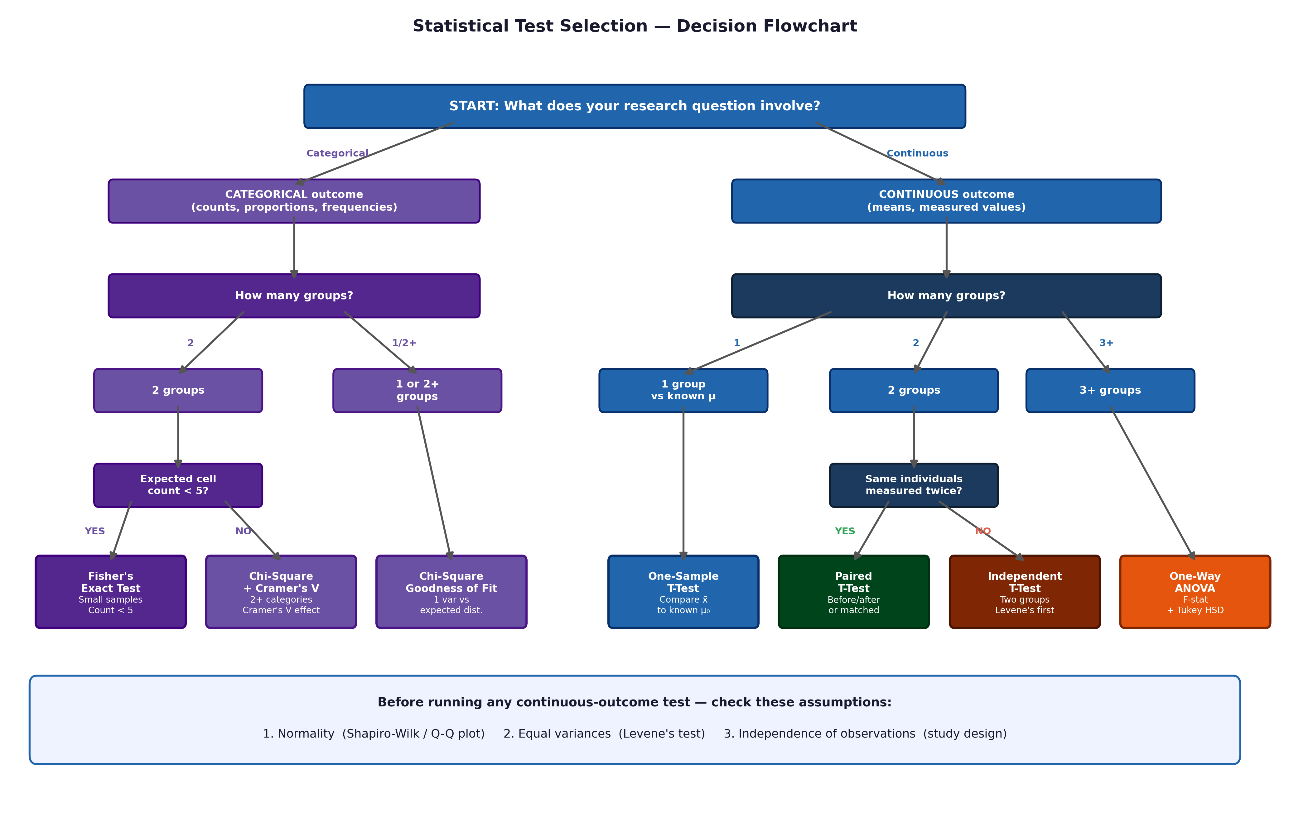
Fig. 25 Figure 9.1 Statistical test selection flowchart. Follow the branches: outcome type → groups → independence → assumptions. All tests in this course appear as leaf nodes.#
The Four-Step Decision Guide#
Step 1 — Outcome type?
Continuous (ratio/interval) \(\rightarrow\) Step 2
Categorical (nominal/ordinal) \(\rightarrow\) Chi-Square or Fisher’s Exact (Step 4)
Time-to-event (censored) \(\rightarrow\) Kaplan-Meier + log-rank test
Step 2 — How many groups?
One (vs known value) \(\rightarrow\) One-Sample T-Test
Two groups \(\rightarrow\) Step 3
Three or more \(\rightarrow\) One-Way ANOVA + Tukey’s HSD
Step 3 — Independent or paired?
Independent (different individuals, e.g., smokers vs non-smokers) \(\rightarrow\) Independent Samples T-Test
Paired (same individuals measured twice, e.g., baseline vs follow-up weight) \(\rightarrow\) Paired Samples T-Test
Step 4 — Assumptions satisfied?
Check Normality (\(n \geq 30 \rightarrow\) CLT applies; \(n < 30 \rightarrow\) Shapiro-Wilk + histogram)
Check equal variances (Levene’s test)
Violated \(\rightarrow\) Non-parametric alternative (Mann-Whitney U, Wilcoxon, Kruskal-Wallis)
For relationships:
Association only \(\rightarrow\) Pearson’s r (or Spearman for skewed/ordinal data)
Prediction \(\rightarrow\) Simple linear regression (non-censored continuous outcome only)
Time-to-event \(\rightarrow\) Kaplan-Meier + log-rank
APA Reporting Templates#
One-sample t-test:
Mean TOTCHOL (M = 235, SD = 42) was significantly higher than the reference of 200 mg/dL, t(499) = 18.6, p < .001, 95% CI [231, 239], d = 0.83.
Independent t-test (Welch’s):
Smokers (M = 133.2, SD = 22.4) had significantly higher SYSBP than non-smokers (M = 130.1, SD = 21.5), t(488.5) = 1.97, p = .049, 95% CI [0.02, 6.2], d = 0.14. (Note the decimal degrees of freedom typical of Welch’s correction).
Paired t-test:
Patients’ body weight significantly increased from baseline (M = 82.4, SD = 5.1) to follow-up (M = 85.1, SD = 5.8) after the intervention, t(71) = 4.12, p < .001, d = 0.49.
One-way ANOVA:
A one-way ANOVA revealed a significant effect of education level on TOTCHOL, F(3, 496) = 4.12, p = .007, η² = .02. Tukey’s HSD indicated [specific pairs].
Chi-Square:
A Chi-Square test of independence indicated a significant association between smoking and CHD incidence, χ²(1, N = 500) = 14.8, p < .001, V = .17.
Pearson correlation:
There was a significant positive correlation between age and systolic blood pressure, r(498) = .38, p < .001, 95% CI [.30, .45].
Log-rank test:
Kaplan-Meier analysis indicated that smokers had significantly shorter survival times than non-smokers, log-rank χ²(1) = 4.1, p = .042.
Part III — Software Cheat Sheets#
PSPP Cheat Sheet#
Analysis |
Menu Path |
|---|---|
Descriptives |
Analyze \(\rightarrow\) Descriptive Statistics \(\rightarrow\) Descriptives |
Median / CI |
Analyze \(\rightarrow\) Descriptive Statistics \(\rightarrow\) Explore |
Histogram |
Graphs \(\rightarrow\) Chart Builder \(\rightarrow\) Histogram |
Normality |
Analyze \(\rightarrow\) Explore \(\rightarrow\) Plots \(\rightarrow\) tick Normality |
One-sample t |
Analyze \(\rightarrow\) Compare Means \(\rightarrow\) One-Sample T Test |
Independent t |
Analyze \(\rightarrow\) Compare Means \(\rightarrow\) Independent-Samples T Test |
Paired t |
Analyze \(\rightarrow\) Compare Means \(\rightarrow\) Paired-Samples T Test |
One-Way ANOVA |
Analyze \(\rightarrow\) Compare Means \(\rightarrow\) One-Way ANOVA |
Chi-Square |
Analyze \(\rightarrow\) Crosstabs \(\rightarrow\) Statistics \(\rightarrow\) Chi-Square |
Correlation |
Analyze \(\rightarrow\) Correlate \(\rightarrow\) Bivariate |
Regression |
Analyze \(\rightarrow\) Regression \(\rightarrow\) Linear |
R Cheat Sheet#
# ── Load data ─────────────────────────────────────────
fram_data <- read.csv("data/framingham_teaching.csv")
library(MASS); data(anorexia)  # Experimental dataset

# ── Factor conversions ────────────────────────────────
fram_data$SEX      <- factor(fram_data$SEX, levels=c(1,2), labels=c("Male","Female"))
fram_data$EDUC     <- factor(fram_data$EDUC, levels=1:4, ordered=TRUE,
  labels=c("0-11yrs","HS_GED","Some_college","College_grad"))
fram_data$CURSMOKE <- factor(fram_data$CURSMOKE, levels=c(0,1), labels=c("Non-smoker","Smoker"))
fram_data$DIABETES <- factor(fram_data$DIABETES, levels=c(0,1), labels=c("No","Yes"))
fram_data$ANYCHD   <- factor(fram_data$ANYCHD,   levels=c(0,1), labels=c("No_CHD","CHD_event"))
fram_data$DEATH    <- factor(fram_data$DEATH,    levels=c(0,1), labels=c("Survived","Died"))

# ── Descriptives ──────────────────────────────────────
summary(fram_data)
tapply(fram_data$SYSBP, fram_data$CURSMOKE, mean)

# ── SE and CI ─────────────────────────────────────────
t.test(fram_data$SYSBP)

# ── Normality ─────────────────────────────────────────
hist(fram_data$SYSBP)
qqnorm(fram_data$SYSBP); qqline(fram_data$SYSBP)
shapiro.test(fram_data$SYSBP)

# ── One-sample t ──────────────────────────────────────
t.test(fram_data$TOTCHOL, mu = 200)

# ── Independent t ─────────────────────────────────────
library(car)
leveneTest(SYSBP ~ CURSMOKE, data = fram_data)
t.test(SYSBP ~ CURSMOKE, data = fram_data)

# ── Paired t ──────────────────────────────────────────
t.test(anorexia$Postwt, anorexia$Prewt, paired = TRUE)

# ── One-Way ANOVA ─────────────────────────────────────
anova_res <- aov(TOTCHOL ~ EDUC, data = fram_data)
summary(anova_res); TukeyHSD(anova_res)

# ANOVA for Anorexia Weight Gain
anorexia$Weight_Change <- anorexia$Postwt - anorexia$Prewt
anova_anorexia <- aov(Weight_Change ~ Treat, data = anorexia)

# ── Chi-Square and proportions ────────────────────────
tbl <- table(fram_data$CURSMOKE, fram_data$ANYCHD)
chisq.test(tbl)
prop.test(tbl)   # Two-proportion z-test + RD/RR from prop.table

# ── Correlation ───────────────────────────────────────
cor.test(fram_data$AGE, fram_data$SYSBP, method="pearson")
cor.test(fram_data$CIGPDAY, fram_data$TOTCHOL, method="spearman")

# ── Regression ────────────────────────────────────────
model <- lm(SYSBP ~ AGE, data = fram_data)
summary(model); confint(model)
par(mfrow=c(2,2)); plot(model); par(mfrow=c(1,1))

# Regression for Anorexia weights
model_wt <- lm(Postwt ~ Prewt, data = anorexia)

# ── Survival analysis ─────────────────────────────────
library(survival)
surv_obj <- Surv(time = fram_data$TIMEDTH, event = fram_data$DEATH)
km_fit   <- survfit(surv_obj ~ CURSMOKE, data=fram_data)
plot(km_fit, col=c("blue","red"), lwd=2,
     xlab="Days", ylab="Survival probability")
survdiff(surv_obj ~ CURSMOKE, data=fram_data)   # Log-rank test
Part IV — Epidemiological Measures Reference#
Health science courses require familiarity with measures beyond standard test statistics. The following table summarises the key epidemiological measures and where they appear in this course.
Measures of Disease Frequency#
Measure |
Formula |
Framingham example |
|---|---|---|
Incidence rate |
Events / person-time |
155 CHD events / 4000 person-years = 38.8/1000 PY |
Cumulative incidence |
Events / population at risk |
155/500 = 31% over 10 years |
Prevalence |
Cases at one time / population |
PREVCHD: 25/500 = 5% at baseline |
Measures of Association#
Measure |
Formula |
Use |
Study design |
|---|---|---|---|
Risk Difference (RD) |
\(p_1 - p_2\) |
Absolute impact |
Cohort / RCT |
Relative Risk (RR) |
\(p_1 / p_2\) |
Relative impact |
Cohort / RCT |
Odds Ratio (OR) |
\(ad/bc\) |
When RR not available |
Case-control; logistic regression |
Attributable Risk (AR) |
\(RD \times 100\) |
Extra events per 100 exposed |
Cohort |
NNH / NNT |
\(1/RD\) |
Clinical impact |
Cohort / RCT |
OR vs RR: OR \(\approx\) RR when the outcome is rare (< 10%). When common (like CHD at 31%), OR > RR and they should not be used interchangeably.
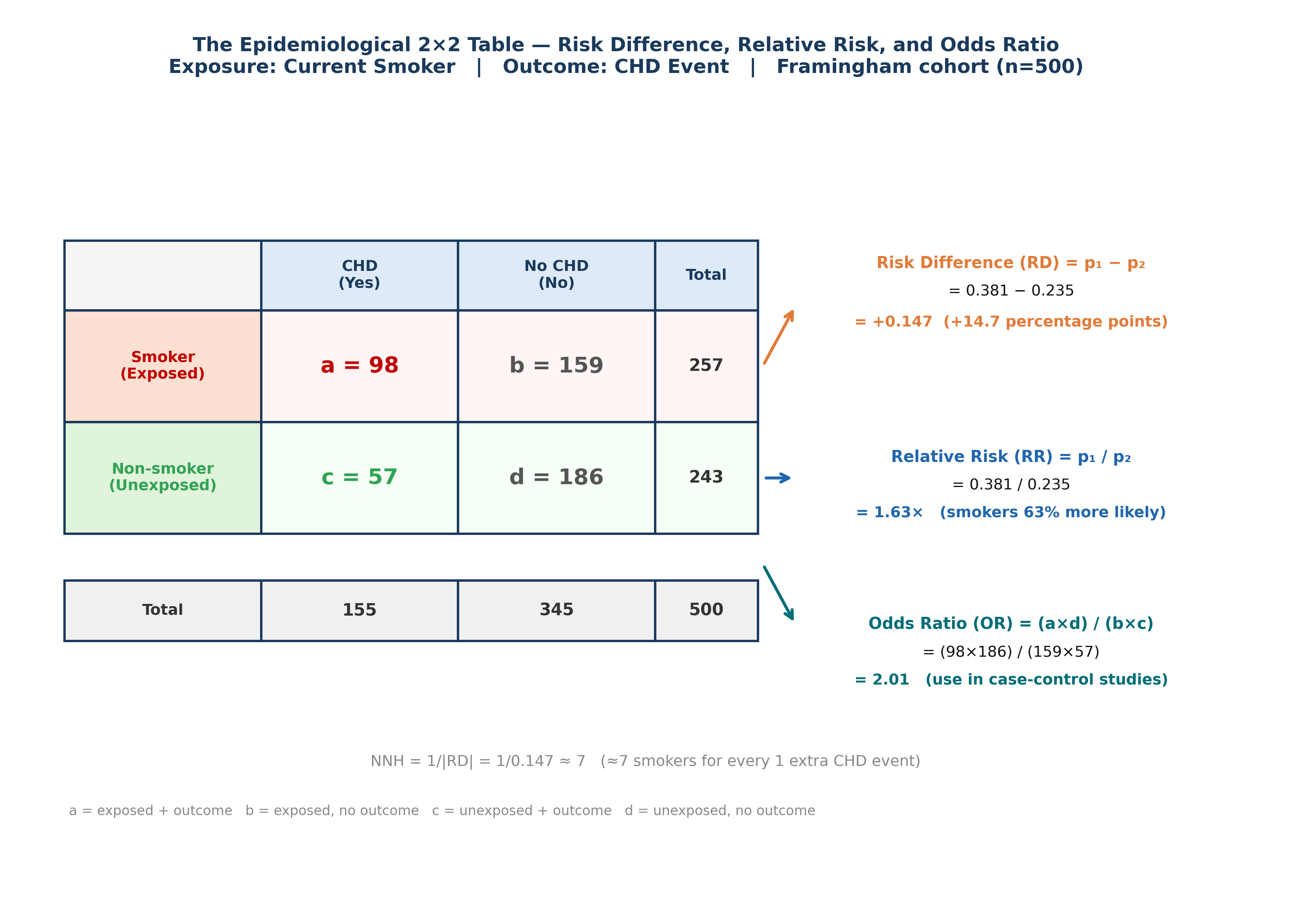
Fig. 26 Figure 9.2 The Epidemiological 2×2 Table — RD, RR, and OR from Real Framingham Data. Smoking (exposure) vs CHD incidence (outcome) across 500 participants. a = smokers with CHD event; b = smokers without; c = non-smokers with CHD; d = non-smokers without. Risk Difference (RD = +14.7 pp): the absolute extra risk from smoking. Relative Risk (RR = 1.63): smokers are 63% more likely to develop CHD. Odds Ratio (OR = 2.01): the case-control equivalent — note OR > RR because CHD is common (31%), so they diverge substantially. NNH ≈ 7: approximately 7 smokers produce 1 extra CHD event.#
Screening and Diagnostic Test Measures#
When a test (e.g., a high-glucose screening test for diabetes) is applied to a population, four measures describe its performance:
Measure |
Formula |
Plain language |
|---|---|---|
Sensitivity (Se) |
True positives / All actual positives |
How good is the test at catching real cases? |
Specificity (Sp) |
True negatives / All actual negatives |
How good is the test at ruling out non-cases? |
Positive Predictive Value (PPV) |
True positives / All test positives |
If the test is positive, how likely is the patient truly positive? |
Negative Predictive Value (NPV) |
True negatives / All test negatives |
If the test is negative, how likely is the patient truly negative? |
Example — glucose screening for diabetes (Framingham context): Suppose we use a glucose threshold of \(\geq 110\) mg/dL to screen for diabetes. The 2×2 table of true diabetes status vs test result would allow calculation of all four measures.
⚡ Common mistake: Sensitivity and specificity are properties of the test. PPV and NPV are properties of the test + the population prevalence. A test with high sensitivity and specificity can have low PPV if disease prevalence is very low (most positives will be false positives).
Study Design Reference#
Design |
Direction |
What you measure |
Key strength |
Key limitation |
|---|---|---|---|---|
RCT / Experimental |
Forward |
Incidence, RR, efficacy |
Randomisation controls confounding |
Expensive; ethical constraints |
Cohort (Observational) |
Forward |
Incidence, RR, survival |
Temporal precedence established |
Time and cost; loss to follow-up |
Case-control |
Backward |
OR (not RR) |
Efficient for rare diseases |
Recall bias; cannot calculate incidence |
Cross-sectional |
Snapshot |
Prevalence, OR |
Fast and cheap |
Cannot establish temporality |
The Framingham Heart Study is a prospective observational cohort, the strongest observational design for identifying risk factors. The Anorexia trial is an Experimental RCT, the gold standard for testing active interventions.
Non-Parametric Equivalents — Quick Reference#
When parametric assumptions are violated (non-Normal data, small samples, or ordinal outcomes), use the non-parametric equivalent. These tests rank the data rather than assuming a specific distribution.
Parametric Test |
When to use it |
Non-Parametric Equivalent |
When to switch |
|---|---|---|---|
One-Sample T-Test |
Continuous outcome vs known value |
Wilcoxon Signed-Rank Test (one-sample) |
\(n < 30\) and non-Normal |
Independent Samples T-Test |
Two unrelated groups, continuous outcome |
Mann-Whitney U Test (Wilcoxon Rank-Sum) |
Non-Normal, small \(n\), or ordinal outcome |
Paired Samples T-Test |
Same individuals measured twice |
Wilcoxon Signed-Rank Test (paired) |
Difference scores non-Normal and \(n < 30\) |
One-Way ANOVA |
Three or more groups, continuous outcome |
Kruskal-Wallis Test |
Non-Normal within groups or ordinal outcome |
Pearson’s r |
Linear association, two continuous variables |
Spearman’s Rho (\(\rho\)) |
Skewed data, outliers, or ordinal variables |
⚡ Common mistake: Many students automatically reach for non-parametric tests whenever data “looks skewed.” Remember the Central Limit Theorem — with \(n \geq 30\) per group, parametric tests are robust to moderate non-Normality. Non-parametric tests have lower statistical power than their parametric equivalents, so switching unnecessarily increases the risk of a Type II error.
In R:
# Mann-Whitney U (independent groups)
wilcox.test(SYSBP ~ CURSMOKE, data = fram_data)

# Wilcoxon signed-rank (paired)
wilcox.test(anorexia$Postwt, anorexia$Prewt, paired = TRUE)

# Kruskal-Wallis (3+ groups)
kruskal.test(TOTCHOL ~ EDUC, data = fram_data)

# Spearman's rho
cor.test(fram_data$AGE, fram_data$SYSBP, method = "spearman")
A Final Word#
In 1948, researchers in Framingham, Massachusetts enrolled 5,209 people and asked: what causes heart disease?
They did not know the answer. They had hypotheses — smoking, diet, stress, genetics — but no definitive proof. What they had was a commitment to measuring carefully, following up rigorously, and applying robust statistical methods to what they found.
Over the next 75 years, the Framingham Heart Study produced over 3,000 publications. It established that high blood pressure damages arteries. It proved that smoking causes heart attacks. It showed that high cholesterol predicts myocardial infarction. It coined the term risk factor. It built the evidence base for every cardiovascular prevention guideline in use today.
But observation is only half the story. Once a public health problem is identified, we must test a solution. That is why this book paired the Framingham cohort with the Anorexia Clinical Trial. The 72 patients in that experimental dataset represent the other pillar of health science: the clinical intervention. When you ran a paired t-test or an ANOVA on their outcomes, you were evaluating the very psychological therapies that save lives and restore well-being.
The statistical methods in this course are not academic exercises. They are the tools that produced that evidence. The t-tests, ANOVA, Chi-Square, regression, and Kaplan-Meier analyses in these chapters are, in their essentials, the exact same analyses that Framingham investigators and clinical researchers rely on every single day.
The participants in our teaching datasets represent real lives. When you calculate the Relative Risk of CHD for smokers, or measure the efficacy of Family Therapy, you are not solving a textbook math problem. You are replicating — in miniature — the analyses that eventually convinced governments to ban smoking in public spaces, shaped modern psychiatric care, and saved millions of lives.
That is what statistics is for.
Key Takeaways
Test selection: outcome type \(\rightarrow\) number of groups \(\rightarrow\) independence \(\rightarrow\) assumptions.
Effect size is always required alongside a p-value.
Survival data (censored) requires KM curves + log-rank, not OLS regression.
Correlation \(\neq\) causation — confounding, reverse causation, and coincidence are always alternatives.
The Datasets: Between the observational Framingham cohort and the experimental Anorexia trial, you have now practiced every core statistical method required in modern health science.
Part IV — Putting It All Together