Chapter 6: A Tale of Two Groups#
Independent and Paired Samples T-Tests#
Datasets:
Framingham Heart Study teaching subset (
framingham_teaching.csv, n = 500) — ObservationalAnorexia Clinical Trial (
anorexiaviaMASSpackage, n = 72) — Experimental
Learning Objectives
By the end of this chapter, you will be able to:
Determine whether a two-group comparison requires an independent or paired t-test.
State and check the assumptions of each test.
Apply Levene’s test and understand Welch’s correction.
Calculate and interpret Cohen’s d for effect size.
Run and interpret both tests in PSPP and R.
Before You Begin: The Research Design Question#
Chapter 5 compared one group to a known value. Most health research, however, compares two groups. Before running any statistical test, one fundamental design question determines everything: are the two groups independent, or related (paired)?
Section 1: Independent vs Paired Designs#
1.1 The Core Distinction#
Independent design: Two completely different groups of unrelated individuals. Framingham example: Do smokers and non-smokers have different mean systolic blood pressure? Each participant appears in exactly one group. This is classic observational epidemiology.
Paired design: The same individuals measured twice, or matched pairs.
Anorexia Clinical Trial example: 72 patients have their body weight measured before (Prewt) and after (Postwt) a psychological intervention. The exact same 72 patients contribute both measurements. This is classic experimental epidemiology.
The decision rule: If the same individual (or a matched pair) contributes to both groups → Paired. If they are completely unrelated individuals → Independent.
⚡ Common mistake: Pre/post measurements on the same patients look like two groups in a spreadsheet, but they are paired. Running an independent t-test on pre/post data discards the pairing, loses statistical power, and can produce the wrong answer.
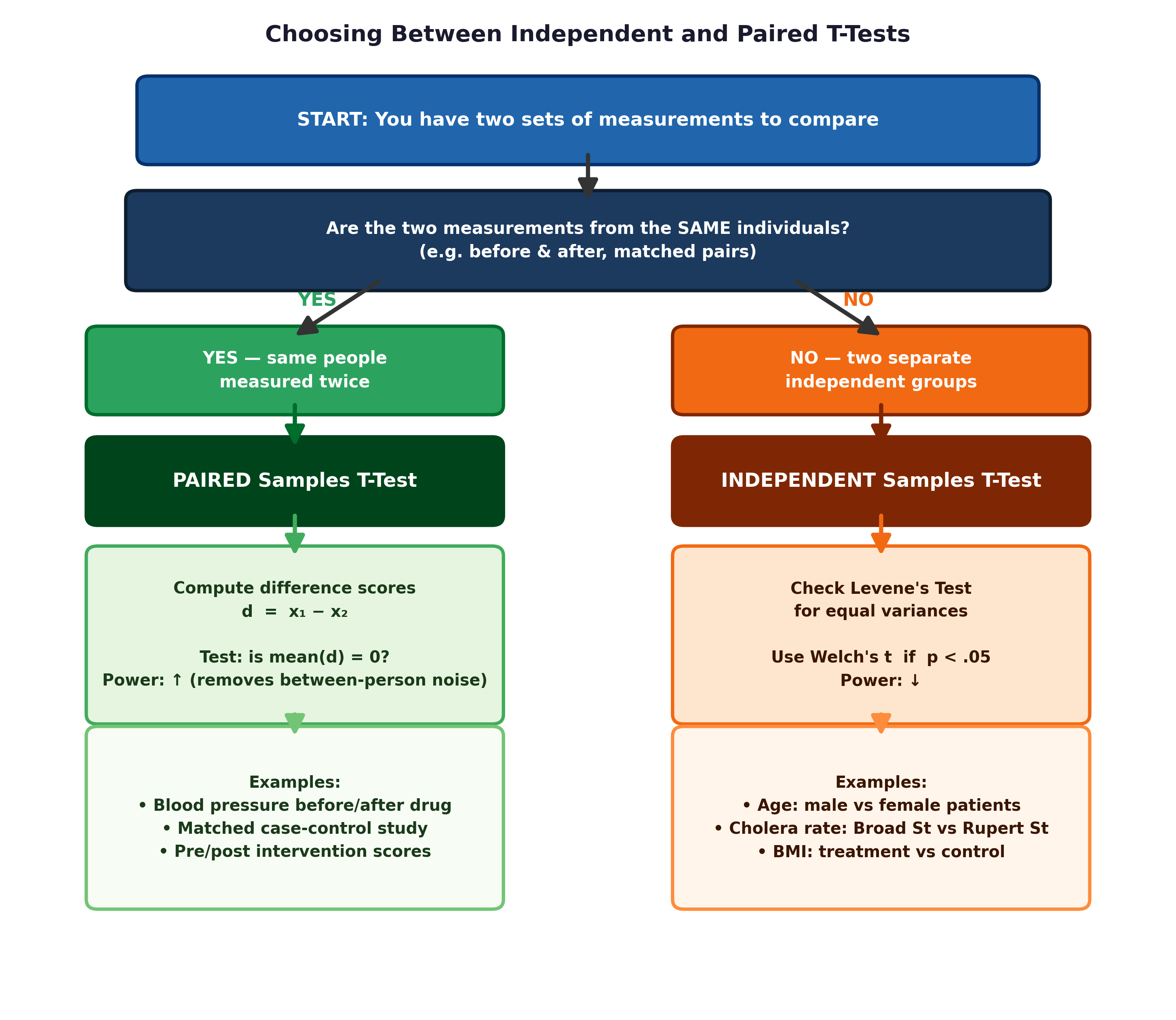
Fig. 16 Figure 6.1 Independent vs paired design. In a paired design, the unit of analysis is the difference score for each individual. This eliminates between-person variability and increases statistical power.#
1.2 Why Pairing Increases Power#
When each participant serves as their own control, all the natural between-person variation (due to genetics, height, baseline metabolism) is removed from the analysis. We are simply asking: did the change in weight differ from zero? Because between-person variability is usually much larger than the treatment effect itself, pairing can dramatically increase statistical power.
Section 2: The Independent Samples T-Test#
2.1 Research Question#
Framingham: Do smokers and non-smokers have different mean systolic blood pressure at baseline?
\(H_0: \mu_{smoker} = \mu_{non-smoker}\)
\(H_1: \mu_{smoker} \neq \mu_{non-smoker}\)
2.2 The Formula (Welch’s Version)#
Note: The formula above is specifically for Welch’s t-test, which does not assume the two groups have equal variances.
2.3 Levene’s Test and Welch’s Correction#
Before interpreting an independent t-test, you must check whether the two groups have similar variances (spread).
Levene’s \(p > 0.05\): Assume equal variances → use the standard pooled-variance t-test.
Levene’s \(p \leq 0.05\): Variances differ significantly → use Welch’s t-test (which adjusts the degrees of freedom to prevent false positives).
💡 The Fractional df Panic: Because it is so robust, R’s
t.test()applies Welch’s correction by default. Welch’s formula applies a mathematical penalty to the degrees of freedom. If you see a decimal for your df in R (e.g., df = 488.5), do not panic! You did not break the software; this is simply the Welch’s correction at work.
2.4 Assumptions#
Assumption |
How to Check |
|---|---|
Independence of groups |
Design-level — verify they are different, unrelated individuals. |
Continuous outcome |
Verify variable is interval or ratio. |
Approximately Normal |
Histogram + Shapiro-Wilk per group (robust if \(n \geq 30\) per group). |
Equal variances |
Levene’s test (use Welch’s correction if violated). |
2.5 Effect Size: Cohen’s d#
A p-value only tells you if a difference exists, not how large or clinically meaningful it is. Cohen’s d measures the standardized difference between two means:
Rule of thumb: \(d = 0.2\) is a small effect, \(0.5\) is medium, and \(0.8\) is large.
Section 3: The Paired Samples T-Test#
💡 Plain English first: A paired t-test is essentially just a one-sample t-test performed on the differences. For each person, calculate (After − Before). Then test whether those difference scores average out to zero.
3.1 Research Question#
To demonstrate the paired t-test, we turn to our experimental anorexia dataset. Patients in a clinical trial had their weight measured at baseline (Prewt) and at the end of the study (Postwt). Did their body weight significantly change?
\(H_0: \mu_{diff} = 0\) (Mean weight change is exactly 0 — no effect of the intervention)
\(H_1: \mu_{diff} \neq 0\)
3.2 The Formula#
For each participant, compute their difference score: \(d_i = \text{after}_i - \text{before}_i\).
Where \(\bar{d}\) = mean of the difference scores, \(s_d\) = standard deviation of the difference scores, and \(n\) = number of pairs.
3.3 Side-by-Side Comparison#
Feature |
Independent T-Test |
Paired T-Test |
|---|---|---|
Groups |
Different individuals |
Same individuals twice (or matched) |
Unit of analysis |
Individual observations |
Difference scores |
df |
\(\approx n_1+n_2-2\) |
\(n-1\) (number of pairs minus 1) |
Power |
Lower |
Higher (removes between-person noise) |
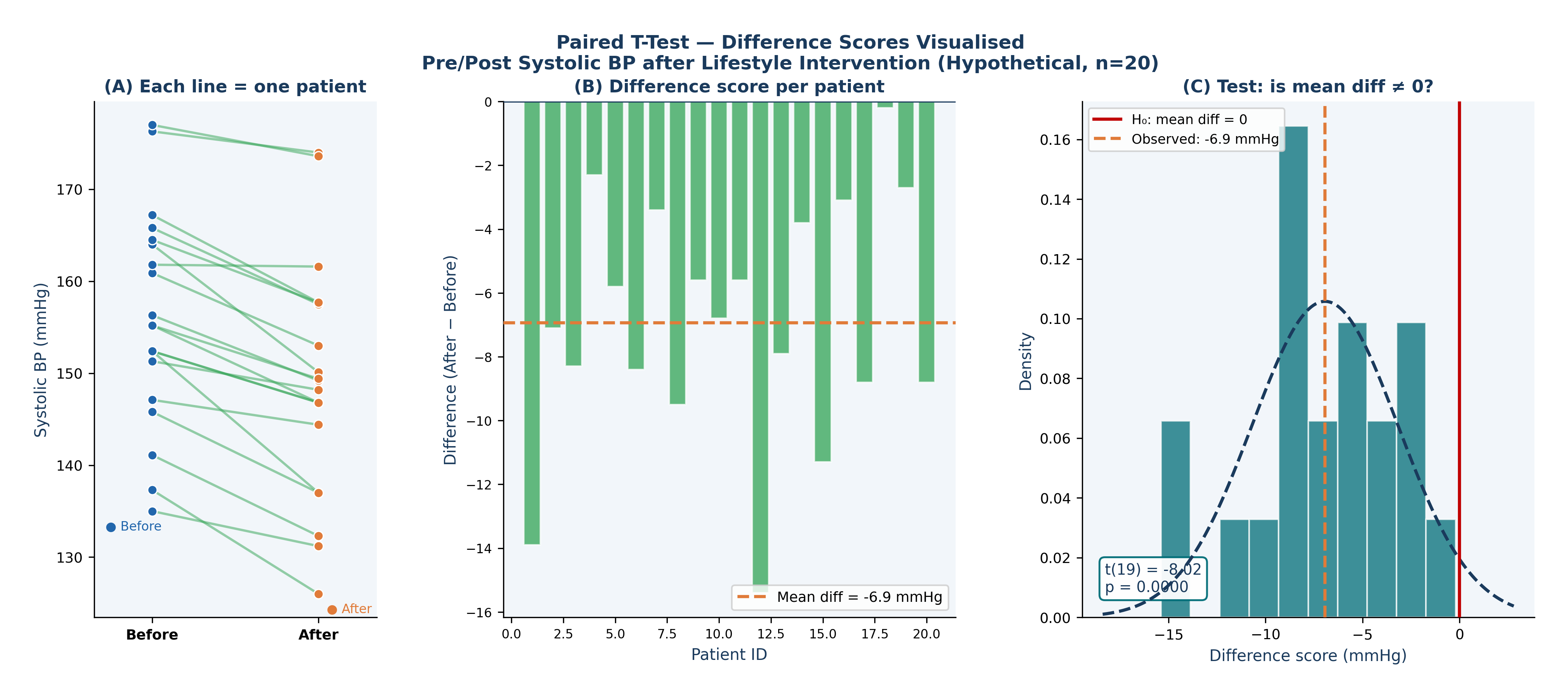
Fig. 17 Figure 6.2 Paired T-Test — Difference Scores Visualised. A hypothetical pre/post lifestyle intervention on 20 hypertensive Framingham participants. (A) Each line connects one patient’s before and after measurement — green lines show BP decreased, red lines show it increased. (B) The difference score (After − Before) for each patient, the orange dashed line marks the mean difference. (C) The paired t-test tests whether the mean of these difference scores is significantly different from zero; t(19) = −8.02, p < 0.001.#
🔬 Lab Manual — Chapter 6#
Objective#
Part 1: Independent t-test — does mean SYSBP differ between smokers and non-smokers in the Framingham cohort? Part 2: Paired t-test — did patient weight significantly change during the Anorexia clinical trial?
Option A — PSPP#
Part 1: Independent t-test (Framingham):
Analyze → Compare Means → Independent-Samples T Test.
Move
SYSBPto Test Variables;CURSMOKEto Grouping Variable.Define Groups: Group 1 = 0, Group 2 = 1. Continue → OK.
Part 2: Paired t-test (Anorexia):
Analyze → Compare Means → Paired-Samples T Test.
Select both
PrewtandPostwtand move them into the “Paired Variables” box.Click OK.
Option B — R / RStudio#
# -------------------------------------------------------
# Chapter 6 Lab: Independent and Paired T-Tests
# -------------------------------------------------------

# ══ Part 1: Independent t-test (Framingham Data) ═════
fram_data <- read.csv("data/framingham_teaching.csv")
fram_data$CURSMOKE <- factor(fram_data$CURSMOKE, levels=c(0,1),
  labels=c("Non-smoker","Smoker"))

# Descriptives by smoking group
tapply(fram_data$SYSBP, fram_data$CURSMOKE, mean, na.rm=TRUE)
tapply(fram_data$SYSBP, fram_data$CURSMOKE, sd, na.rm=TRUE)

# Normality check per group
by(fram_data$SYSBP, fram_data$CURSMOKE, shapiro.test)

# Levene's test
library(car)
leveneTest(SYSBP ~ CURSMOKE, data = fram_data)

# Independent t-test (Welch by default in R)
t.test(SYSBP ~ CURSMOKE, data = fram_data)

# Effect size: Cohen's d
m1 <- mean(fram_data$SYSBP[fram_data$CURSMOKE=="Smoker"],   na.rm=TRUE)
m2 <- mean(fram_data$SYSBP[fram_data$CURSMOKE=="Non-smoker"],na.rm=TRUE)

# Note: Using overall SD as a simplified approximation of pooled SD for beginners
s_pool <- sd(fram_data$SYSBP, na.rm=TRUE)
d <- abs(m1 - m2) / s_pool
cat("Cohen's d =", round(d, 3), "\n")

# Visualise
boxplot(SYSBP ~ CURSMOKE, data = fram_data,
        main = "Systolic BP by Smoking Status",
        xlab = "Smoking Status", ylab = "SYSBP (mmHg)",
        col = c("#BDD7EE","#FEE0D2"))

# ══ Part 2: Paired t-test (Anorexia Data) ════════════
library(MASS)
data(anorexia)

# Calculate difference scores: Weight Change (After - Before)
difference_scores <- anorexia$Postwt - anorexia$Prewt

# Check Normality of DIFFERENCES (not raw values)
shapiro.test(difference_scores)
hist(difference_scores,
     main = "Weight Change in Trial (Postwt − Prewt)",
     xlab = "Change in Weight (lbs)",
     col = "#C7E9C0", border = "white")

# Paired t-test
t.test(anorexia$Postwt, anorexia$Prewt, paired = TRUE)
What to examine:
Independent t-test: Is mean SYSBP higher in smokers than non-smokers? Is the difference statistically significant? Is Cohen’s d \(> 0.2\) (small) or \(> 0.5\) (medium)?
Levene’s test: If \(p < 0.05\), Welch’s correction (the default in R) is appropriate.
Paired t-test: Look at the p-value. Did the patients’ weight significantly change from baseline to follow-up? The paired design eliminates natural variations in height and body type, focusing entirely on whether individuals changed.
🧪 Test Your Knowledge#
Compare mean total cholesterol (TOTCHOL) between diabetic (DIABETES=1) and non-diabetic (DIABETES=0) participants in the Framingham dataset.
(a) Is this an independent or paired design?
(b) State \(H_0\) and \(H_1\).
(c) Run the test and interpret the output, including Cohen’s d.
Show Solution
# (a) Independent — diabetic and non-diabetic participants are two
#     different groups of completely unrelated individuals.

# (b) H_0: \mu_{TOTCHOL(diabetes)} = \mu_{TOTCHOL(no diabetes)}
#     H_1: \mu_{TOTCHOL(diabetes)} \neq \mu_{TOTCHOL(no diabetes)}

# (c) R code:
fram_data$DIABETES <- factor(fram_data$DIABETES, levels=c(0,1),
  labels=c("No diabetes","Diabetes"))

tapply(fram_data$TOTCHOL, fram_data$DIABETES, mean, na.rm=TRUE)
t.test(TOTCHOL ~ DIABETES, data = fram_data)

# Effect size:
m_diab   <- mean(fram_data$TOTCHOL[fram_data$DIABETES=="Diabetes"], na.rm=TRUE)
m_nodiab <- mean(fram_data$TOTCHOL[fram_data$DIABETES=="No diabetes"], na.rm=TRUE)

# Note: Using overall SD as a simplified approximation
d_chol   <- abs(m_diab - m_nodiab) / sd(fram_data$TOTCHOL, na.rm=TRUE)
cat("Cohen's d =", round(d_chol, 3))
Key Terms#
Term |
Definition |
|---|---|
Independent t-test |
Compares the means of two completely unrelated groups. |
Paired t-test |
Compares two measurements from the same individuals or matched pairs. The unit of analysis is the difference score. |
Levene’s test |
Tests equality of variances. \(p > 0.05\) \(\rightarrow\) assume equal variances. |
Welch’s correction |
Safely adjusts the degrees of freedom when group variances are unequal. This is the default in R. |
Difference score (d) |
Per-person change: (After − Before). The paired t-test analyzes these directly. |
Cohen’s d |
A standardized measure of effect size. \(0.2\) = small, \(0.5\) = medium, \(0.8\) = large. |
Review Questions#
A Framingham researcher compares mean BMI between participants with prevalent hypertension and those without. Is this an independent or paired design? State \(H_0\) and \(H_1\), run the test in R, and interpret.
Explain why Welch’s t-test is preferred over the standard equal-variance t-test as a default in modern statistical practice.
In the paired t-test example using the Anorexia dataset, why is the Shapiro-Wilk test applied strictly to the difference scores rather than to the
PrewtandPostwtmeasurements separately?Run
t.test(SYSBP ~ CURSMOKE, data=fram_data)in R. Report the t-statistic, df, p-value, and the 95% CI for the difference. Is the difference clinically meaningful given the overall standard deviation of SYSBP (\(\approx 22\) mmHg)?Explain, using the concept of between-person variability, why a paired t-test for a pre/post weight study will inherently have higher statistical power than an independent t-test comparing the baseline group to the follow-up group.
Key Takeaways
Independent: Two unrelated groups. \(t = (\bar{x}_1 - \bar{x}_2) / SE_{diff}\).
Paired: Same individuals twice. \(t = \bar{d} / (s_d / \sqrt{n})\). Yields higher statistical power.
Levene’s test checks for equal variances. Welch’s correction is a safer default when variances differ.
Never run an independent t-test on pre/post data from the same individuals.
Always report Cohen’s d—a small p-value alone does not mean a finding is clinically important.
Next: Chapter 7 — Scaling Up extends our toolkit to three or more groups and categorical associations.
Part II — Testing What We Think We Know