Chapter 7: Scaling Up

Chapter 7: Scaling Up#

ANOVA, Chi-Square, and Categorical Comparisons#

Datasets:

Framingham Heart Study teaching subset (framingham_teaching.csv, n = 500) — Observational

Anorexia Clinical Trial (anorexia via MASS package, n = 72) — Experimental

Learning Objectives

By the end of this chapter, you will be able to:

Explain the multiple comparisons problem and calculate the FWER.
Run and interpret a one-way ANOVA with Tukey’s HSD post-hoc test.
Compare two proportions and calculate risk difference, relative risk, and odds ratios.
Run and interpret a Chi-Square test and Fisher’s Exact Test.
Calculate and interpret Cramér’s V as an effect size.

Before You Begin: Beyond Two Groups#

Chapters 5 and 6 handled one or two groups. However, health science routinely requires us to compare three or more groups, or to examine whether specific risk factors are associated with disease outcomes. This chapter extends your toolkit in two directions:

Three or more continuous groups → One-Way ANOVA
Two categorical variables → Chi-Square / Fisher’s Exact Test

Section 1: The Multiple Comparisons Problem#

💡 The Intuition: Run enough tests and you will eventually get a “significant” result purely by accident. With an alpha level of $0.05$, every test has a 5% false-positive rate. If you run 14 independent tests, you have a roughly 50% chance of getting at least one false positive.

1.1 Why Repeated T-Tests Fail#

The Framingham dataset includes four education levels (EDUC = 1, 2, 3, 4). To compare mean cholesterol across all four groups using t-tests, you would need to run six separate pairwise comparisons (Group 1 vs 2, 1 vs 3, 1 vs 4, etc.).

Every time you run a test, risk accumulates. This is called the Family-Wise Error Rate (FWER):

\[FWER = 1 - (1 - \alpha)^k\]

With $k = 6$ comparisons and $\alpha = 0.05$, the FWER becomes $1 - 0.95^6 \approx 0.26$. This means you have a 26% chance of making a Type I error—more than five times the intended risk!

1.2 The Solution: One Protected Analysis#

ANOVA solves this problem. Instead of running six risky t-tests, ANOVA performs a single “omnibus” test comparing all groups simultaneously. This protects your Type I error rate, keeping it locked at exactly $\alpha = 0.05$.

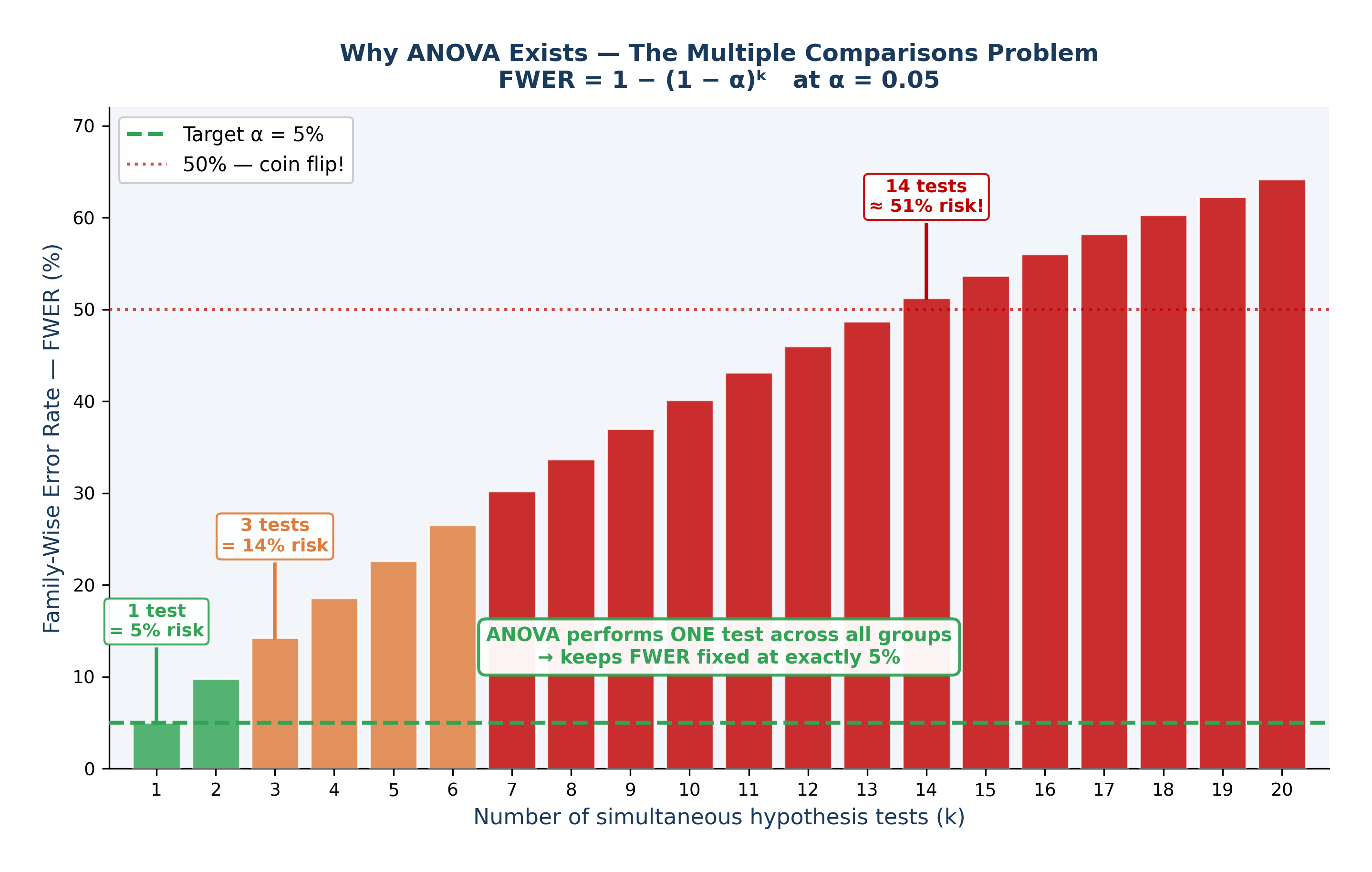
../_images/ch07_fwer_inflation.png — Fig. 18 **Figure 7.3 The Multiple Comparisons Problem — FWER Inflation.** Family-Wise Error Rate (FWER) = 1 − (1 − α)ᵏ at α = 0.05. With just 1 test the false positive risk is the intended 5% (green). By 3 tests it reaches 14% (orange). By 14 tests it exceeds 50%, a worse-than-coin-flip chance of at least one false positive (red). ANOVA solves this by performing a single omnibus test across all groups, keeping FWER fixed at exactly 5%.#

Section 2: One-Way ANOVA#

2.1 Research Questions#

Observational (Framingham): Does mean total cholesterol (TOTCHOL) differ across the four education levels? Experimental (Anorexia): Does mean weight gain (Weight_Change) differ across the three psychological treatment groups (CBT, Family Therapy, Control)?

$H_0: \mu_1 = \mu_2 = \mu_3 = ...$ (All group means are equal)
$H_1:$ At least one group mean differs from the others

2.2 The F-Statistic: How Variance Tells Us About Means#

It sounds contradictory: why is it called Analysis of Variance (ANOVA) when we are testing means?

Imagine looking at three groups of patients. ANOVA breaks the total variation in the data into two parts:

Between-Group Variance (The Signal): How far apart are the group averages from each other?
Within-Group Variance (The Noise): How scattered are the individual patients within their own groups?

\[F = \frac{MS_{Between}}{MS_{Within}} = \frac{\text{Signal}}{\text{Noise}}\]

If F $\approx$ 1: The differences between the groups are no larger than the random noise within the groups. We fail to reject $H_0$.
If F >> 1: The groups are spread far apart relative to their internal noise. The signal is real. We reject $H_0$.

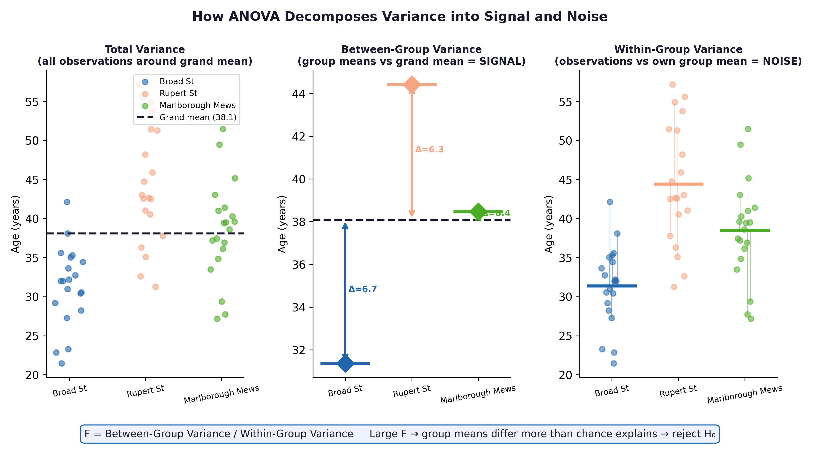
../_images/ch07_anova_decomposition.png — Fig. 19 **Figure 7.1** ANOVA decomposes total variance into between-group variance (signal) and within-group variance (noise). In the Framingham context, between-group variance captures genuine cholesterol differences linked to education; within-group variance captures individual biological variation unrelated to education.#

Effect size: $\eta^2$ (Eta-Squared) $$\eta^2 = \frac{SS_{Between}}{SS_{Total}}$$ This tells us the proportion of total variance explained by the groups. *Rule of thumb:* $\eta^2 = 0.01$ is small, $0.06$ is medium, $0.14$ is large.

2.3 Post-Hoc Tests — Tukey’s HSD#

A significant ANOVA F-test only tells you that at least one group is different. It does not tell you which one.

To find out, we use Tukey’s Honest Significant Difference (HSD). Tukey’s safely compares all specific pairs (e.g., CBT vs Control, CBT vs FT) while mathematically suppressing the Family-Wise Error Rate.

⚡ Crucial Rule: Only apply Tukey’s HSD after you get a significant overall ANOVA result. Digging for differences after a non-significant ANOVA is invalid.

2.4 Assumptions#

Assumption	How to Check It
Independence	Verified by study design (no repeated measures here).
Normal Distribution	Histogram or Shapiro-Wilk test per group. (ANOVA is very robust to violations if $n > 30$ per group).
Homogeneity of Variances	Levene’s test. If violated, use a Welch ANOVA instead.

Section 3: Comparing Two Proportions#

Research question: Is the proportion of patients who develop Coronary Heart Disease (ANYCHD) different between smokers and non-smokers?

To compare two event rates ($p_1$ and $p_2$), we use different effect sizes depending on our study design. Understanding the difference between them is vital for public health communication.

Risk Difference (RD): $p_1 - p_2$. The absolute difference in proportions.
Relative Risk (RR): $p_1 / p_2$. A multiplier showing how many times more likely the event is in the exposed group.
Odds Ratio (OR): $(a \times d) / (b \times c)$. The ratio of the odds of an event occurring in one group to the odds of it occurring in another group.

Epidemiological interpretation: Suppose smokers have a 38% CHD incidence and non-smokers have a 25% incidence.

Measure	Formula	Result	Plain Language Translation
Risk Difference (RD)	$p_1 - p_2$	38% − 25% = +13%	There are 13 extra cases of CHD per 100 smokers.
Relative Risk (RR)	$p_1 / p_2$	38 / 25 = 1.52	Smokers are 52% more likely to develop CHD.
Number Needed to Harm (NNH)	$1 / RD$	1 / 0.13 = 7.7	On average, for every 8 people who smoke, 1 “extra” CHD event will occur. (Note: RD must be input as a decimal, e.g., 0.13, not 13).

⚡ Common mistake: Relative Risk (RR) can only be calculated from cohort studies or clinical trials where you know the total population at risk (like the Framingham study). In a case-control study (where researchers artificially select a set number of sick and healthy people), you cannot calculate risk. You must use the Odds Ratio (OR) instead.

Section 4: Chi-Square Tests#

4.1 Research Question#

Framingham: Is there a statistically significant association between smoking status (CURSMOKE) and CHD incidence (ANYCHD)?

$H_0:$ Smoking and CHD are completely independent (no association).
$H_1:$ Smoking and CHD are associated.

4.2 The Contingency Table#

	ANYCHD = 0 (No event)	ANYCHD = 1 (Event)	Total
Non-smoker	a	b	a+b
Smoker	c	d	c+d
Total	a+c	b+d	n

4.3 Expected Counts: The “Perfectly Fair” World#

To calculate a Chi-Square statistic, we compare the data we actually observed ($O$) to the data we would have expected ($E$) if the null hypothesis were perfectly true.

If smoking had absolutely no effect on heart disease, then the overall background rate of CHD (say, 31%) should apply equally to both smokers and non-smokers. The expected count represents this mathematically fair, null-hypothesis world:

\[\text{Expected Count} = \frac{\text{Row Total} \times \text{Column Total}}{n}\]

The Chi-Square formula simply measures how far our observed reality deviates from that null expectation:

\[\chi^2 = \sum \frac{(O - E)^2}{E}\]

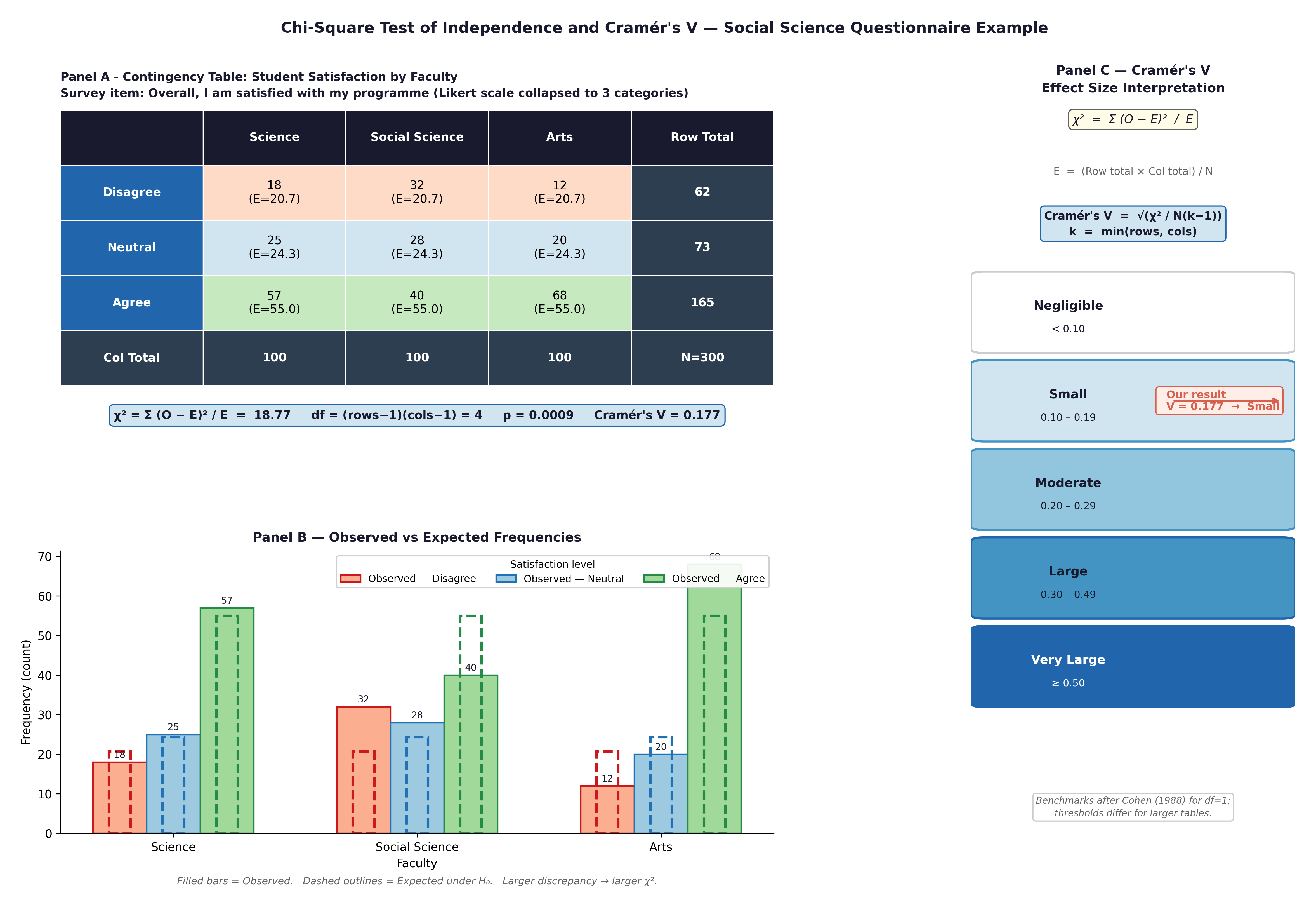
../_images/ch07b_chisquare_cramers_v.png — Fig. 20 **Figure 7.2** Chi-Square test components: contingency table with observed and expected counts, grouped bar chart of proportions, and Cramér’s V interpretation scale.#

⚡ Crucial Rule: Chi-Square mathematics break down if your sample is too small. It requires expected counts to be $\geq 5$ in every single cell of your table. If this fails, you must use Fisher’s Exact Test instead. PSPP and R will warn you, but it is your responsibility to check.

Effect size: Cramér’s V $$V = \sqrt{\frac{\chi^2}{n \times (\min(r,c)-1)}}$$ *Rule of thumb:* $V < 0.1$ is negligible; $0.10 - 0.29$ is small; $0.30 - 0.49$ is moderate; $\geq 0.50$ is large.

🔬 Lab Manual — Chapter 7#

Objective#

Part 1: ANOVA — Does mean total cholesterol differ across education levels? Does therapy type affect weight gain? Part 2: Chi-Square — Is smoking associated with CHD incidence? Part 3: Proportions — Calculate RR, RD, and OR for smoking and CHD.

Option A — PSPP#

ANOVA: Analyze → Compare Means → One-Way ANOVA. TOTCHOL as Dependent, EDUC as Factor. Post Hoc → Tukey. Options → Homogeneity of variance test.

Chi-Square: Analyze → Descriptive Statistics → Crosstabs. CURSMOKE as Row, ANYCHD as Column. Statistics → Chi-Square + Phi and Cramér’s V. Cells → Observed, Expected, Row percentages.

Option B — R / RStudio#

# -------------------------------------------------------
# Chapter 7 Lab: ANOVA and Chi-Square
# -------------------------------------------------------

fram_data <- read.csv("data/framingham_teaching.csv")

# install.packages("car") # <-- Run this line once if you do not have the 'car' package
library(car)

fram_data$EDUC <- factor(fram_data$EDUC, levels=1:4,
  labels=c("0-11yrs","HS_GED","Some_college","College_grad"), ordered=TRUE)
fram_data$CURSMOKE <- factor(fram_data$CURSMOKE, levels=c(0,1),
  labels=c("Non-smoker","Smoker"))
fram_data$ANYCHD <- factor(fram_data$ANYCHD, levels=c(0,1),
  labels=c("No_CHD","CHD_event"))

# ══ Part 1a: One-Way ANOVA (Framingham Data) ═════════

tapply(fram_data$TOTCHOL, fram_data$EDUC, mean, na.rm=TRUE)
tapply(fram_data$TOTCHOL, fram_data$EDUC, sd, na.rm=TRUE)

leveneTest(TOTCHOL ~ EDUC, data = fram_data)

anova_result <- aov(TOTCHOL ~ EDUC, data = fram_data)
summary(anova_result)

# Effect size: eta-squared
SS <- summary(anova_result)[[1]]$"Sum Sq"
eta_sq <- SS[1] / sum(SS)
cat("eta-squared =", round(eta_sq, 3), "\n")

TukeyHSD(anova_result)

boxplot(TOTCHOL ~ EDUC, data = fram_data,
        main = "Total Cholesterol by Education Level",
        xlab = "Education", ylab = "TOTCHOL (mg/dL)",
        col = c("#FEE0D2","#FDD0A2","#C7E9C0","#BDD7EE"))

# ══ Part 1b: One-Way ANOVA (Anorexia Trial Data) ═════

library(MASS)
data(anorexia)

# First, calculate the outcome variable: Weight Gain
anorexia$Weight_Change <- anorexia$Postwt - anorexia$Prewt

# Run ANOVA to compare weight gain across the 3 therapy groups
anova_anorexia <- aov(Weight_Change ~ Treat, data = anorexia)
summary(anova_anorexia)
TukeyHSD(anova_anorexia)

# ══ Part 2: Chi-Square (Framingham Data) ═════════════

tbl <- table(fram_data$CURSMOKE, fram_data$ANYCHD)
print(tbl)

# Check expected counts (all should be >= 5)
chi_result <- chisq.test(tbl)
print(chi_result$expected)
print(chi_result)

# Cramér's V
V <- sqrt(chi_result$statistic / (sum(tbl) * (min(dim(tbl))-1)))
cat("Cramér's V =", round(V, 3), "\n")

# ══ Part 3: Proportions and RR ═══════════════════════

prop.table(tbl, margin=1)    # Row proportions

# Relative Risk and Risk Difference
p_smoke   <- tbl["Smoker","CHD_event"] / sum(tbl["Smoker",])
p_nosmoke <- tbl["Non-smoker","CHD_event"] / sum(tbl["Non-smoker",])
RD <- p_smoke - p_nosmoke
RR <- p_smoke / p_nosmoke

cat("CHD rate — smokers:    ", round(p_smoke*100,1), "%\n")
cat("CHD rate — non-smokers:", round(p_nosmoke*100,1), "%\n")
cat("Risk Difference:", round(RD*100,1), "percentage points\n")
cat("Relative Risk:  ", round(RR,2), "\n")

What to examine:

ANOVA (Framingham): Does TOTCHOL significantly differ by education level? Which specific pairs differ in Tukey’s HSD? Is $\eta^2$ small, medium, or large?
ANOVA (Anorexia): Did the type of psychological therapy significantly impact weight gain? Look at the Tukey results to see which specific therapy (FT or CBT) outperformed the Control group.
Chi-Square: Is there a statistically significant association between smoking and CHD? Is Cramér’s V large enough to be clinically meaningful?

Worked Example — CHD Risk in Smokers vs Non-smokers#

Using the Framingham dataset, suppose our $2 \times 2$ table shows:

	CHD event	No CHD event	Total
Smoker	98	157	255
Non-smoker	57	188	245
Total	155	345	500

Step 1 — Proportions:

$p_{smoker} = 98 / 255 = 38.4\%$
$p_{non-smoker} = 57 / 245 = 23.3\%$

Step 2 — Risk Difference: $38.4\% - 23.3\% = \textbf{+15.1 percentage points}$ → Smoking is associated with 15 extra CHD events per 100 people over the study period.

Step 3 — Relative Risk: $38.4 / 23.3 = \textbf{1.65}$ → Smokers are 65% more likely to develop CHD.

Step 4 — Odds Ratio: $(98 \times 188) / (157 \times 57) = 18424 / 8949 = \textbf{2.06}$ → Note: Because CHD is common in this cohort, the OR (2.06) diverges substantially from the RR (1.65). If this were a case-control study, we would calculate this cross-product ratio instead of the RR.

Step 5 — Number Needed to Harm (NNH): $1 / 0.151 = \textbf{6.6}$ → On average, about 7 smokers will develop a CHD event that would not have occurred in a non-smoker. (Note how we divided by the decimal 0.151, not the percentage).

Step 6 — Chi-Square test:

Expected counts are all $\geq 5$ ✓
$\chi^2(1) = 14.8, p < 0.001$
Cramér’s V = 0.17 (small-to-moderate association)

🧪 Test Your Knowledge#

Test whether body mass index (BMI) differs across the four education groups using ANOVA. (a) State $H_0$ and $H_1$. (b) Run the ANOVA and Tukey’s HSD. (c) Calculate $\eta^2$ and interpret it. (d) Based on the pattern, does education appear to be a social determinant of BMI in this cohort?

Key Terms#

Term	Definition
FWER	Family-Wise Error Rate — the probability of $\geq 1$ false positive across $k$ comparisons.
One-Way ANOVA	Tests whether $\geq 3$ group means differ. F = between-variance / within-variance.
Tukey’s HSD	Post-hoc test safely comparing all group pairs after a significant ANOVA.
$\eta^2$ (eta-squared)	ANOVA effect size. The proportion of variance explained by the group categories.
Risk Difference	$p_1 - p_2$. The absolute difference in event proportions.
Relative Risk (RR)	$p_1 / p_2$. Multiplicative comparison of event rates between two groups.
Odds Ratio (OR)	$(a \times d) / (b \times c)$. Ratio of odds. Used in case-control studies where RR cannot be calculated.
Chi-Square test	Tests the independence of two categorical variables. Requires expected counts $\geq 5$.
Fisher’s Exact Test	The required alternative to Chi-Square when expected cell counts are $< 5$.
Cramér’s V	Chi-Square effect size. $0$ = no association, $1$ = perfect association.

Review Questions#

Calculate the FWER for 6 pairwise comparisons at $\alpha = 0.05$. Why is ANOVA preferable to running all 6 t-tests?
Run aov(SYSBP ~ EDUC, data=fram_data) and TukeyHSD() in R. Which education groups differ in mean systolic blood pressure? Interpret the pattern.
Using the Anorexia dataset, run aov(Weight_Change ~ Treat, data = anorexia) and perform TukeyHSD(). Which specific psychological therapy proved significantly better at increasing patient weight than the Control group?
A Chi-Square test comparing smoking status and death returns $\chi^2(1) = 4.8$, $p = 0.028$, Cramér’s V = 0.10. Write a complete one-paragraph interpretation.
Calculate the Relative Risk (RR) for the association between prevalent hypertension (PREVHYP) and any CHD event (ANYCHD). Interpret the result in plain clinical language.
Run chisq.test(table(fram_data$BPMEDS, fram_data$ANYCHD)). Check the expected cell counts. Are they all $\geq 5$? If not, which test should you use instead, and why?

Key Takeaways

ANOVA protects your Type I error rate when comparing $\geq 3$ means.
$F$ = Signal / Noise. A significant $F$ means you can run Tukey’s HSD to find specific differences.
$\eta^2$: $< 0.06$ small, $0.06 - 0.14$ medium, $> 0.14$ large.
Relative Risk (RR) and Risk Difference (RD) quantify the epidemiological burden of a risk factor.
Chi-Square tests categorical associations by comparing Observed vs Expected counts. If Expected cells are $< 5$, you must use Fisher’s Exact Test.

Next: Chapter 8 — Reading the Future introduces correlation, regression, and survival analysis.

Part III — Comparing More Than Two Groups

Measure	Formula	Result	Plain Language Translation
Risk Difference (RD)	\(p_1 - p_2\)	38% − 25% = +13%	There are 13 extra cases of CHD per 100 smokers.
Relative Risk (RR)	\(p_1 / p_2\)	38 / 25 = 1.52	Smokers are 52% more likely to develop CHD.
Number Needed to Harm (NNH)	\(1 / RD\)	1 / 0.13 = 7.7	On average, for every 8 people who smoke, 1 “extra” CHD event will occur. (Note: RD must be input as a decimal, e.g., 0.13, not 13).