Chapter 5: The Hypothesis Gamble#
Hypothesis Testing, P-Values, and Statistical Power#
Dataset: Framingham Heart Study teaching subset —
framingham_teaching.csv, n = 500 participants.
Learning Objectives
By the end of this chapter, you will be able to:
Formulate null and alternative hypotheses for a clinical research question.
Describe probability and non-probability sampling methods.
Interpret a p-value correctly, and identify the four most common misinterpretations.
Define Type I and Type II errors and explain the trade-off between them.
Explain statistical power and the four factors that increase it.
Run and interpret a one-sample t-test.
Before You Begin: The Logic of the Trial#
Chapters 1 through 4 described data. Hypothesis testing asks a fundamental new question: is this finding real, or could it have occurred by chance?
This framework underpins every clinical trial, every drug approval, and every public health policy decision based on epidemiological evidence. It is also the most widely misunderstood framework in applied science. This chapter aims to teach it correctly.
Section 1: Sampling — The Foundation of Inference#
1.1 The Target Population and the Sampling Frame#
Target population — everyone you want to draw conclusions about (e.g., all middle-aged adults at cardiovascular risk in Western populations).
Study population — the subset you can actually reach (e.g., residents of Framingham, Massachusetts, 1948–1968).
Sample — the 500 participants we are working with.
Sampling frame — the mechanism used to select the sample (in Framingham, a near-complete census of eligible Framingham residents).
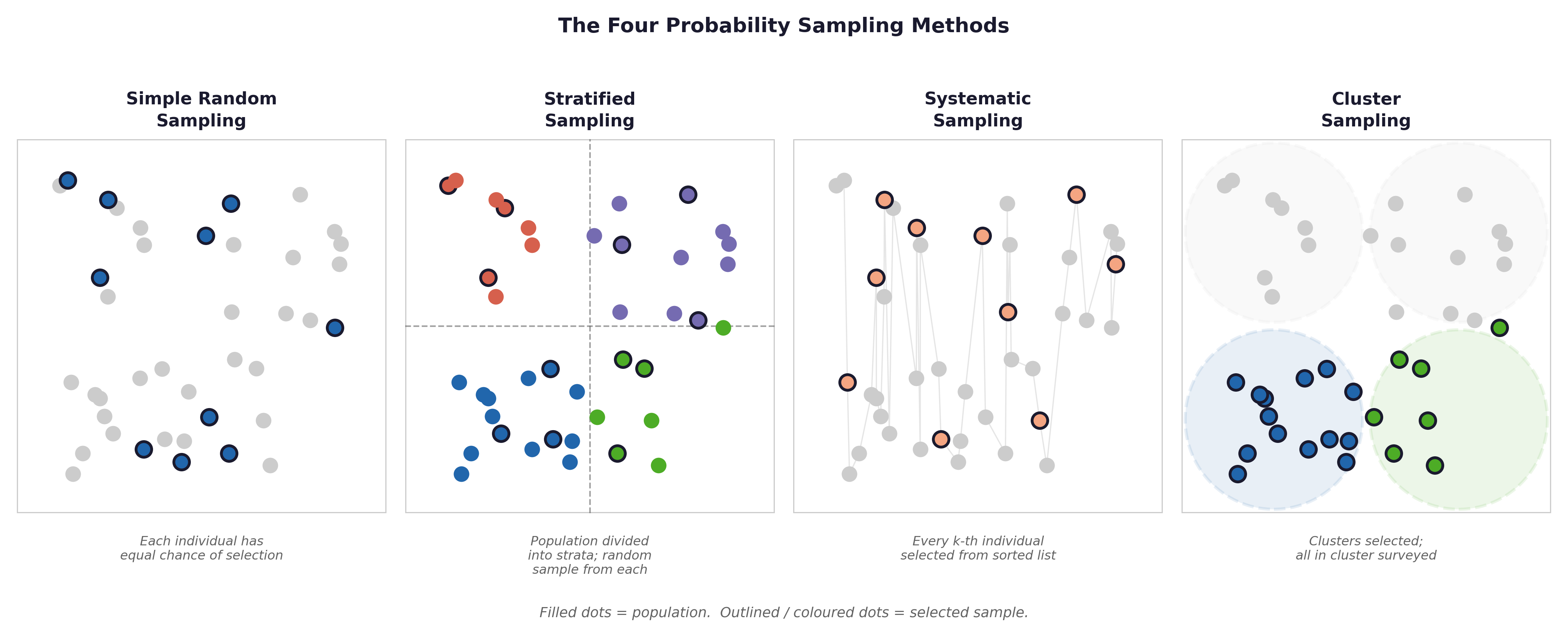
Fig. 12 Figure 5.1 Four probability sampling methods (simple random, stratified, systematic, cluster) and three non-probability methods (convenience, purposive, snowball). The Framingham study used a near-census approach — close to simple random sampling within eligible age bands. This is why its findings generalise well to similar populations.#
1.2 Probability Sampling Methods#
Method |
How it works |
Framingham relevance |
|---|---|---|
Simple random |
Every individual has equal selection probability |
Framingham approximated this within age-eligible residents |
Stratified |
Random sample from defined subgroups |
Used in modern Framingham offspring cohorts by age/sex strata |
Systematic |
Every kth individual selected from a list |
Used in some large registry studies |
Cluster |
Entire groups selected randomly |
Used in national surveys (e.g., NHANES) |
1.3 Non-Probability Methods#
Method |
Description |
Limitation |
|---|---|---|
Convenience |
Whoever is available |
May not represent the target population |
Purposive |
Deliberately selected for specific characteristics |
Not generalisable beyond selected group |
Snowball |
Participants recruit other participants |
Network-dependent selection bias |
The Framingham limitation: The original cohort was almost entirely White, from one Massachusetts town. This is a form of selection bias. Despite the study’s size and rigour, its risk factor estimates may not apply equally to all ethnic and geographic populations, a limitation the investigators acknowledged explicitly.
1.4 Epidemiological Study Designs#
The choice of statistical test depends partly on the study design that generated the data. Three designs appear in most health science research.
Design |
How it works |
What you can calculate |
Framingham example |
|---|---|---|---|
Cohort study |
Follow a group forward in time from exposure to outcome |
Incidence, RR, hazard ratio |
Framingham itself — 500 participants followed for 10 years |
Case-control study |
Start from outcomes, look backward at exposures |
Odds Ratio (OR) — not RR directly |
Compare CHD cases vs matched controls on smoking history |
Cross-sectional study |
Measure exposure and outcome at the same time |
Prevalence, OR |
A single Framingham examination visit — everyone measured once |
💡 Plain English: Cohort studies follow people forward (exposure → outcome). Case-control studies work backward (outcome → who had the exposure?). Cross-sectional studies are a snapshot — everyone measured at one moment.
The Framingham Heart Study is a prospective cohort study, the gold standard for identifying risk factors. Risk factors were measured at baseline before heart disease developed, which establishes temporal precedence (an important criterion for causality).
⚡ Common mistake: Cohort studies give Relative Risk (RR). Case-control studies give Odds Ratio (OR). In rare diseases, OR \(\approx\) RR, but for common outcomes like CHD (31% in Framingham), they differ substantially. Always identify the study design before choosing which effect measure to report.
Section 2: The Framework of the Trial#
2.1 The Presumption of No Effect#
Hypothesis testing begins from a default position: nothing interesting is happening. Any observed difference is assumed to be due to chance until the data persuades us otherwise.
2.2 The Two Competing Hypotheses#
💡 Plain English first: Think of hypothesis testing like a court trial. \(H_0\) (“innocent until proven guilty”) is assumed true until the data provides sufficient evidence to reject it. \(H_1\) is the prosecution’s case.
Null hypothesis (\(H_0\)): No effect, no difference, no association. Any observed result is due to chance.
Alternative hypothesis (\(H_1\)): A real effect, difference, or association exists.
Worked example — Framingham SYSBP: The WHO defines normal systolic blood pressure as 120 mmHg. Is the mean SYSBP of our Framingham cohort different from this reference value?
\(H_0: \mu_{SYSBP} = 120\) mmHg
\(H_1: \mu_{SYSBP} \neq 120\) mmHg (two-tailed — we have not specified a direction)
We assume \(H_0\) is true and ask: if the true population mean really were 120 mmHg, how likely would we be to observe a sample mean as far from 120 as we did (\(\bar{x} \approx 131.6\) mmHg)?
2.3 One-Tailed and Two-Tailed Tests#
Two-tailed: \(H_1: \mu \neq 120\). We test whether SYSBP differs in either direction.
One-tailed: \(H_1: \mu > 120\). We predict a specific direction before seeing the data.
Default: Use two-tailed tests unless there is a pre-registered, theory-driven justification for one direction. In the cardiovascular context, testing whether a cohort from the 1950s has higher BP than the modern reference is directionally intuitive, but two-tailed remains the conservative and more defensible choice.
Section 3: The P-Value#
3.1 What It Measures#
The p-value is the probability of obtaining a result at least as extreme as the one observed, assuming \(H_0\) is true.
If the true mean SYSBP were really 120 mmHg, how often would we draw a random sample of 500 participants with a mean as far from 120 as 131.6 mmHg? If this probability is very small, we doubt \(H_0\) is true.
3.2 The Significance Threshold (\(\alpha\))#
The significance level (\(\alpha\)) is the threshold below which we reject \(H_0\). Conventionally \(\alpha = 0.05\).
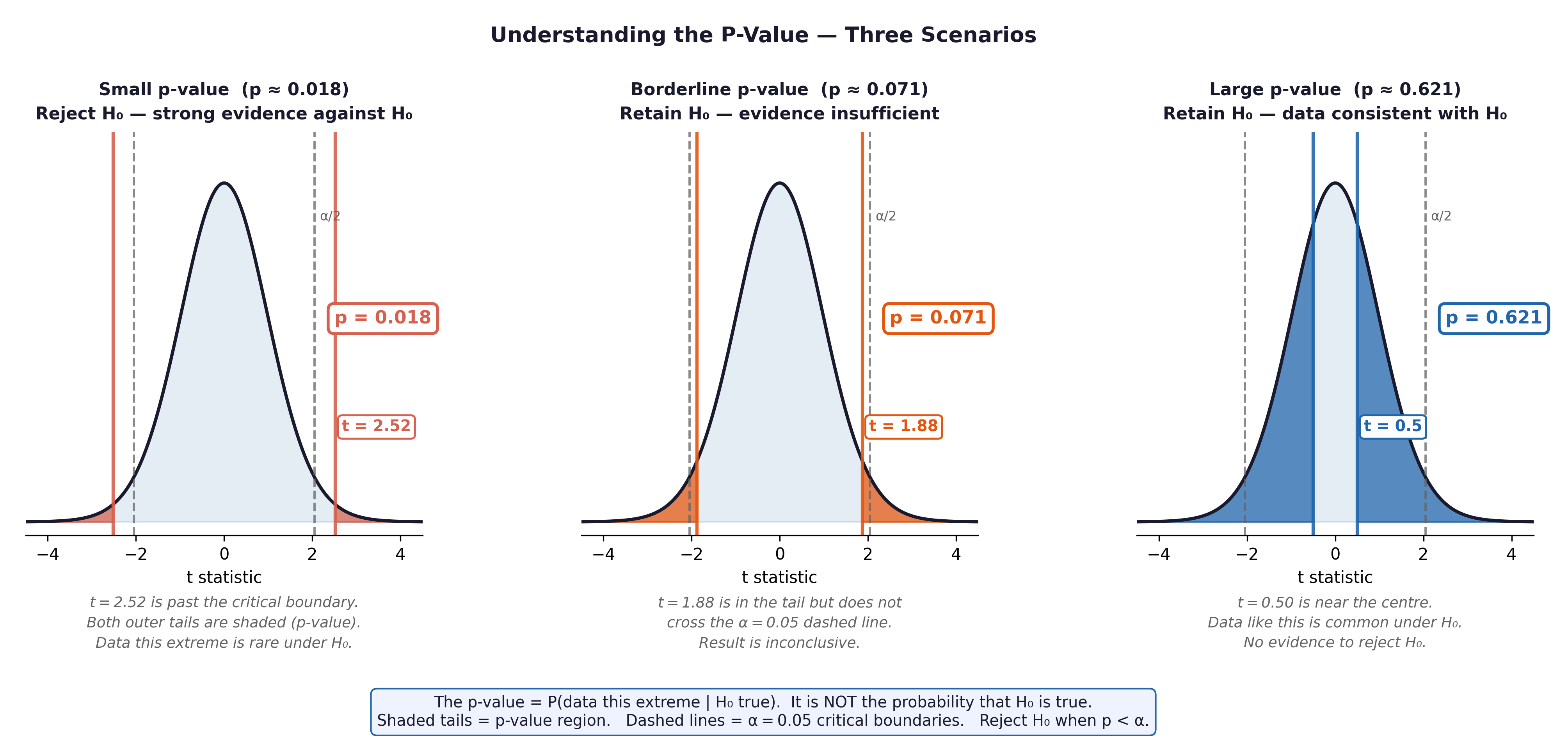
Fig. 13 Figure 5.2 The p-value concept. The shaded tails represent the probability of observing a result as extreme as ours (or more extreme) if H₀ were true. When p < 0.05 (shaded area < 5%), we reject H₀.#
3.3 What the P-Value Does NOT Mean#
❌ Misinterpretation |
✅ What is actually true |
|---|---|
“p is the probability \(H_0\) is true” |
p assumes \(H_0\) is true — it cannot evaluate whether \(H_0\) is true |
“p = 0.03 means 3% chance result is due to chance” |
Same error, different wording |
“p = 0.001 means the effect is large or important” |
Small p = strong evidence against \(H_0\), not large effect size |
“p = 0.06 means the result is not real” |
It means evidence did not reach threshold — study may be underpowered |
⚡ Common mistake: Always report an effect size alongside the p-value. In the Framingham context, \(p < 0.001\) for mean SYSBP vs 120 mmHg is not surprising with \(n = 500\) — any small, potentially clinically trivial deviation from 120 will be statistically significant.
Section 4: Type I and Type II Errors#
Setting \(\alpha = 0.05\) means we accept two possible errors with opposite causes and opposite remedies.
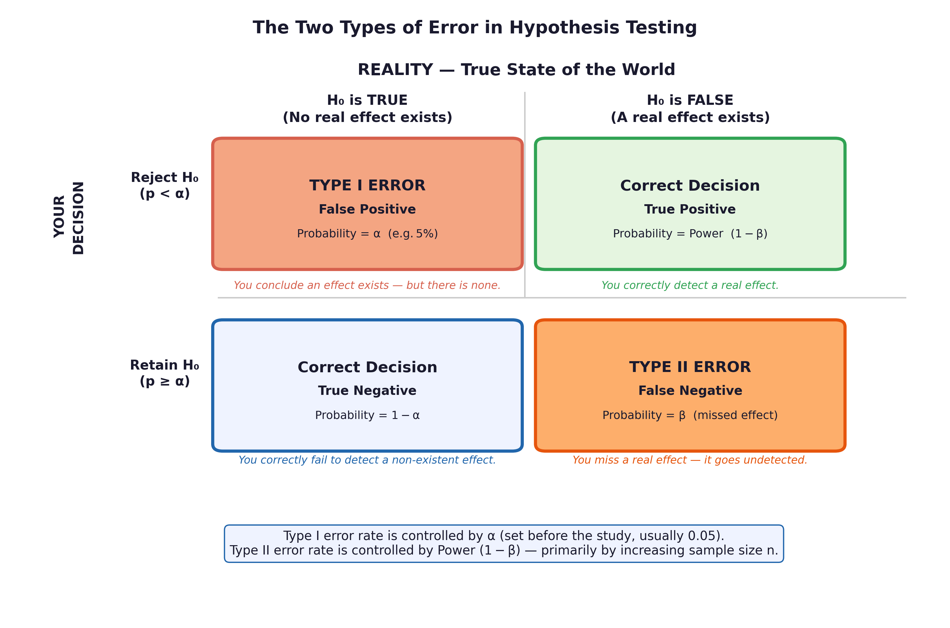
Fig. 14 Figure 5.3 Type I and Type II errors. Type I (false positive) = rejecting a true H₀. Type II (false negative) = failing to reject a false H₀.#
\(H_0\) actually TRUE |
\(H_0\) actually FALSE |
|
|---|---|---|
We REJECT \(H_0\) |
❌ Type I error (\(\alpha\)) |
✅ Correct (Power = \(1-\beta\)) |
We FAIL TO REJECT \(H_0\) |
✅ Correct |
❌ Type II error (\(\beta\)) |
Cardiovascular example:
Type I error: A drug trial concludes a new antihypertensive works when it does not. Patients receive an ineffective treatment.
Type II error: A drug trial concludes a new antihypertensive does not work when it does. An effective treatment is abandoned.
The consequences are asymmetric. In the Framingham era, Type II errors were common — underpowered studies missed real associations between smoking and heart disease before the evidence accumulated to irrefutable levels.
Section 5: Statistical Power#
Statistical power (\(1 - \beta\)) is the probability of detecting a real effect when one exists.
Conventional minimum: power \(\geq 0.80\) (80%).
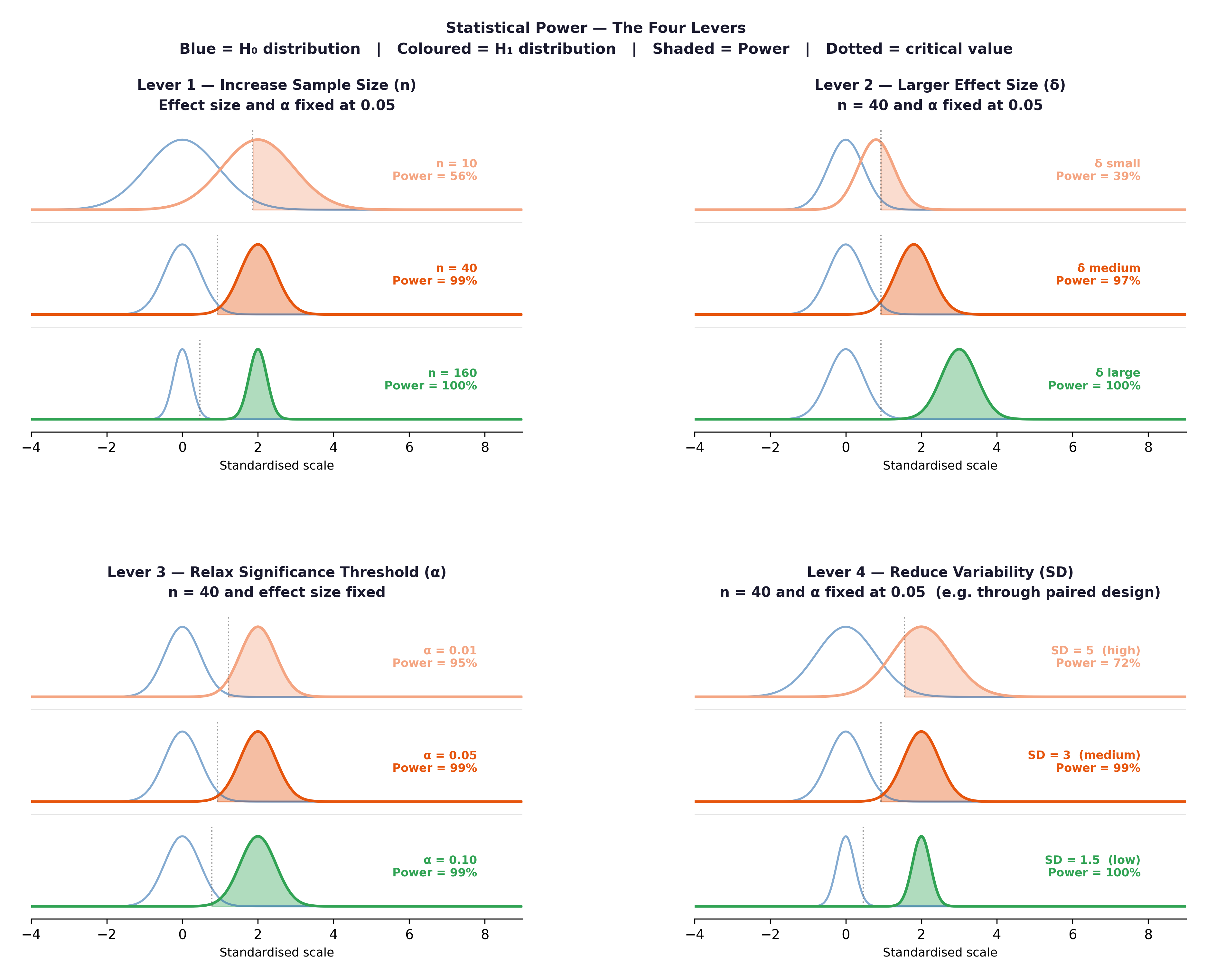
Fig. 15 Figure 5.4 The four levers of statistical power. Increasing any of these raises power and reduces Type II error risk.#
The four levers:
Increase n, the most reliable lever. Framingham’s 5,209 original participants gave enormous power to detect modest risk factor effects.
Increase effect size; if the true difference is larger, it is easier to detect.
Decrease \(\sigma\) — more precise measurements reduce noise.
Increase \(\alpha\) — raising from 0.05 to 0.10 increases power but also Type I error risk.
Section 6: The One-Sample T-Test#
6.1 When to Use It#
The one-sample t-test tests whether the mean of a sample differs from a known population value (\(\mu_0\)).
Requirements: Continuous ratio/interval variable; approximately Normal or \(n \geq 30\); representative sample.
Research question: Is the mean systolic BP of the Framingham cohort significantly different from the reference value of 120 mmHg?
\(H_0: \mu_{SYSBP} = 120\)
\(H_1: \mu_{SYSBP} \neq 120\)
6.2 The T-Statistic#
6.3 Reading the Output#
t-statistic and df (degrees of freedom = \(n - 1\))
p-value — is the result statistically significant at \(\alpha = 0.05\)?
95% CI for the mean — does it include \(\mu_0 = 120\)?
Sample mean and Cohen’s d — is the difference clinically meaningful?
🔬 Lab Manual — Chapter 5#
Objective#
Test whether mean SYSBP in the Framingham cohort differs from the reference value of 120 mmHg. Interpret all output elements.
Option A — PSPP#
Analyze → Compare Means → One-Sample T Test.
Move
SYSBPto Test Variables. Set Test Value = 120. Click OK.
Option B — R / RStudio#
# -------------------------------------------------------
# Chapter 5 Lab: One-Sample T-Test
# H₀: mean SYSBP = 120 mmHg   H₁: mean SYSBP ≠ 120 mmHg
# -------------------------------------------------------

fram_data <- read.csv("data/framingham_teaching.csv")

# ── Descriptives first ────────────────────────────────
mean(fram_data$SYSBP, na.rm = TRUE)
sd(fram_data$SYSBP, na.rm = TRUE)

hist(fram_data$SYSBP,
     main = "Distribution of Systolic Blood Pressure",
     xlab = "SYSBP (mmHg)", col = "#BDD7EE", border = "white")

# ── Normality check ───────────────────────────────────
shapiro.test(fram_data$SYSBP)

# ── One-sample t-test ─────────────────────────────────
t.test(fram_data$SYSBP, mu = 120)

# ── Effect size: Cohen's d ────────────────────────────
# Using abs() ensures the effect size is positive for easy comparison
d <- abs(mean(fram_data$SYSBP, na.rm = TRUE) - 120) / sd(fram_data$SYSBP, na.rm = TRUE)
cat("Cohen's d =", round(d, 3), "\n")
# d < 0.2 = trivial, 0.2-0.5 = small, 0.5-0.8 = medium, > 0.8 = large

# ── Also test TOTCHOL vs reference of 200 mg/dL ───────
t.test(fram_data$TOTCHOL, mu = 200)
d_chol <- abs(mean(fram_data$TOTCHOL, na.rm = TRUE) - 200) / sd(fram_data$TOTCHOL, na.rm = TRUE)
cat("TOTCHOL Cohen's d =", round(d_chol, 3), "\n")
What to examine:
Is \(p < 0.05\)? Almost certainly — with \(n = 500\), even a small deviation from 120 will be significant.
Does the 95% CI include 120 mmHg? If not, the result is significant.
What is Cohen’s d? A statistically significant result with \(d < 0.2\) is clinically trivial. A \(d > 0.5\) means the cohort’s mean BP is substantially elevated.
🧪 Test Your Knowledge#
The published mean TOTCHOL for “desirable” cardiovascular health is 200 mg/dL. Test whether the Framingham cohort’s mean cholesterol differs from this reference. (a) State \(H_0\) and \(H_1\). (b) Run the test. (c) Interpret the p-value, 95% CI, and Cohen’s d. Is the difference clinically significant as well as statistically significant?
Show Solution
# (a) H_0: \mu_{TOTCHOL} = 200 mg/dL
#     H_1: \mu_{TOTCHOL} \neq 200 mg/dL

# (b) R code:
t.test(fram_data$TOTCHOL, mu = 200)

# (c) Expected result: mean ≈ 235 mg/dL — 35 mg/dL above the reference.
#     p will be < 0.001 with n=500.
#     95% CI will not include 200 mg/dL.
#     Cohen's d = abs(235-200)/42 ≈ 0.83 — LARGE effect size.
#     This is both statistically AND clinically significant: the average
#     Framingham participant had cholesterol in the "borderline high" range.
#     This finding contributed to cholesterol's identification as a CVD risk factor.
d_chol <- abs(mean(fram_data$TOTCHOL, na.rm=TRUE) - 200) / sd(fram_data$TOTCHOL, na.rm=TRUE)
cat("Cohen's d =", round(d_chol, 3))
Key Terms#
Term |
Definition |
|---|---|
\(H_0\) (null hypothesis) |
Assumption of no effect. Assumed true until data provides sufficient evidence otherwise. |
\(H_1\) (alternative hypothesis) |
The claim that a real effect exists. |
P-value |
Probability of observing a result as extreme as ours, assuming \(H_0\) is true. |
\(\alpha\) (significance level) |
Threshold below which \(H_0\) is rejected. Conventionally 0.05. |
Type I error |
Rejecting a true \(H_0\) (false positive). Probability = \(\alpha\). |
Type II error |
Failing to reject a false \(H_0\) (false negative). Probability = \(\beta\). |
Statistical power |
\(1-\beta\). Probability of detecting a real effect when one exists. |
Cohen’s d |
Effect size for t-tests. $d = |
Review Questions#
State \(H_0\) and \(H_1\) for the following: “Is the mean diastolic blood pressure in the Framingham cohort different from the reference value of 80 mmHg?”
The one-sample t-test for mean SYSBP vs 120 mmHg returns \(t(499) = 11.8\), \(p < 0.001\). A student writes: “There is less than 0.1% probability that blood pressure is normal in this cohort.” Correct this misinterpretation precisely.
Run
t.test(fram_data$AGE, mu = 50)in R. Interpret the output fully, including the 95% CI and Cohen’s d.The Framingham TOTCHOL test returns \(p < 0.001\), Cohen’s \(d = 0.83\). Explain why both statistics are needed for a complete interpretation.
The Framingham original cohort was almost entirely White. How does this affect the Type I and Type II error rates when the findings are applied to diverse populations?
Key Takeaways
\(H_0\) is assumed true until data provides sufficient evidence to reject it.
p-value: probability of the data given \(H_0\), not the probability \(H_0\) is true.
Type I error (\(\alpha\)): false positive. Type II error (\(\beta\)): false negative. They trade off.
Power (\(1-\beta\)): increased by larger \(n\), larger effect size, lower variance, or higher \(\alpha\).
Effect size (Cohen’s d): essential alongside p-value — statistical significance \(\neq\) clinical importance.
Next: Chapter 6 — A Tale of Two Groups extends the t-test to compare two independent or paired groups.
Part II — Testing What We Think We Know